Proceedings of the Twenty-Eighth AAAI Conference on Artificial Intelligence
Efficient Optimization for Autonomous
Robotic Manipulation of Natural Objects
Abdeslam Boularias and J. Andrew Bagnell and Anthony Stentz
The Robotics Institute, Carnegie Mellon University, Pittsburgh, PA 15213 USA
{Abdeslam, dbagnell, tony}@andrew.cmu.edu
Abstract
Manipulating natural objects of irregular shapes, such as
rocks, is an essential capability of robots operating in outdoor environments. Physics-based simulators are commonly
used to plan stable grasps for man-made objects. However,
planning is an expensive process that is based on simulating hand and object trajectories in different configurations,
and evaluating the outcome of each trajectory. This problem
is particularly concerning when the objects are irregular or
cluttered, because the space of feasible grasps is significantly
smaller, and more configurations need to be evaluated before
finding a good one. In this paper, we first present a learning technique for fast detection of an initial set of potentially
stable grasps in a cluttered scene. The best detected grasps
are further optimized by fine-tuning the configuration of the
hand in simulation. To reduce the computational burden of
this last operation, we model the outcomes of the grasps as a
Gaussian Process, and use an entropy-search method in order
to focus the optimization on regions where the best grasp is
most likely to be. This approach is tested on the task of clearing piles of real, unknown, rock debris with an autonomous
robot. Empirical results show a clear advantage of the proposed approach when the time window for decision is short.
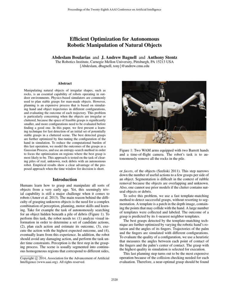
Figure 1: Two WAM arms equipped with two Barrett hands
and a time-of-flight camera. The robot’s task is to autonomously remove all the rocks in the pile.
or facets, of the objects (Szeliski 2011). This step narrows
down the number of useful actions to a few grasps per side of
an object. Segmentation is difficult in the context of rubble
removal because the objects are overlapping and unknown.
Also, one cannot use prior models if the clutter contains natural objects or debris.
To solve this problem, we use a fast template-matching
method to detect successful grasps, without resorting to segmentation. A template is a patch in the depth image, containing the points that may collide with the hand. A large number
of templates were collected and labeled. The outcome of a
grasp is predicted by its k-nearest neighbor templates.
The best grasps detected by the template-matching technique are further optimized by varying the robotic hand’s rotation and the angles of its fingers. Trajectories of the palm
and the fingers are simulated with different configurations.
To evaluate the quality of a configuration, we use a heuristic
that measures the angles between each point of contact of
the fingers and the palm’s center of contact. The grasp with
the highest quality in simulation is selected for execution.
This last planning step turns out to be the most expensive
operation because of the collision checking needed for each
evaluation. Therefore, a near-optimal grasp should be found
Introduction
Humans learn how to grasp and manipulate all sorts of
objects from a very early age. Yet, this seemingly trivial capability is still a major challenge when it comes to
robots (Amor et al. 2013). The main reason behind the difficulty of grasping unknown objects is the need for a complex
combination of perception, planning, motor skills and learning. Take for example the task of autonomously searching
for an object hidden beneath a pile of debris (Figure 1). To
perform this task, the robot needs to: (1) analyze visual information in order to determine a set of candidate actions,
(2), plan each action and estimate its outcome, (3), execute the action with the highest expected outcome, and (4),
eventually learn from this experience. In addition, the robot
should avoid any damaging action, and perform the task under time constraints. Perception is the first step in the grasping process. The scene is usually segmented into continuous homogeneous regions that correspond to different sides,
c 2014, Association for the Advancement of Artificial
Copyright Intelligence (www.aaai.org). All rights reserved.
2520
Get a depth
image of a
clutter from an
RGB-D sensor
Sample a large
number of
random grasps
Learning:
Simulate each
sampled grasp
and label it
Insert the
collision
surfaces and
the labels in
a cover tree
Testing:
Predict the
qualities of the
grasps using
k-NN with
the training
cover tree
Simulate and
optimize the
best predicted
grasps under
a time budget
Extract the
collision
surface of
each grasp
Plan the arm
trajectory
and execute
the predicted
best grasp
Figure 2: Overview of the approach. The learning and the testing mechanisms are both automated, with no human supervision.
define S(x, y) as the average z-coordinate of the points in
cell (x, y). For cells (x, y) with no points (due to occlusions
for example), we set S(x, y) to a default value, corresponding to the average of S in all cells that contain points. Figure 3(b) shows a collision surface represented as a function.
with a minimum number of evaluations. We cast this problem in the Bayesian optimization framework (Jones, Schonlau, and Welch 1998; Lizotte 2008; Tesch, Schneider, and
Choset 2013). Specifically, we model the grasp quality function as a Gaussian Process (GP) (Rasmussen and Williams
2005), and calculate a distribution on the best grasp. The
grasps are evaluated in the order of their contributions to the
entropy of this distribution, which is updated after each evaluation, until a time limit is reached. Figure 2 illustrates the
pipeline of the proposed approach. There are two separate
processes, learning and testing.
We use three-fingered robotic hands; two fingers are always maintained in parallel and point to the opposite direction of the thumb (Figure 1). We define a grasping configuration by (~a, θ, d, c), where ~a is the approach direction of
the hand (the palm’s normal vector), θ is the rotation angle
of the hand, d is the initial distance between the tips of the
fingers (the opening), and c is the contact point, obtained by
projecting the palm’s center on the clutter in the direction ~a.
Planning
To simulate the trajectories of the robotic hand and fingers,
we implemented a 3-D model of the Barrett hand using the
Point Cloud Library (PCL) (Rusu and Cousins 2011). Time
is discretized to short steps. The hand moves in direction
~a towards contact point c, with a constant velocity. Upon
touching the surface, the fingers start closing. Collisions
with the clutter are checked at every time-step. Any collision stops the motion of the palm, as well as the parts of the
fingers involved in the collision.
To measure the quality of a grasp (~a, θ, d, c) at the final
time-step of the simulated motion, we use a simple heuristic that we found useful in our experiments. For each finger i, we search for the point p∗i on its surface that max.(pi −c)T
imizes h(pi ) = ~akp
. The grasp quality is given by
i −ck2
P
∗
h(p
).
For
example,
a grasp is maximally stai
i∈{1,2,3}
ble when each finger circulates the object, i.e. (p∗i − c) k ~a
and h(p∗i ) = ~a.~a = 1. Another example is when finger i is
blocked by clutter above of c and h(p∗i ) becomes negative.
Planning is performed by varying one or more of the initial parameters (~a, θ, d, c), and simulating the corresponding
grasps. The grasp with the highest value is retained.
Feature extraction
A grasp quality measure is a function of different features
of the hand, the object, and the surrounding clutter (Suárez,
Roa, and Cornella 2006). These features include mechanical
properties of objects, such as inertia matrices and friction
factors. Due to the difficulty of inferring mechanical properties of unknown objects from visual input, we consider only
geometric features. These features are obtained by projecting a three-dimensional model of the hand onto the point
cloud, and retaining all the points that may collide with the
hand when it is fully open (blue strips in Figure 3(a)). We
call this set a collision surface.
The collision surface is transformed to a standard frame,
relative to the hand. This frame is defined by setting c, the
palm center projected on the cloud, as the origin, the thumb’s
direction as the x-axis and the approach direction as the
z-axis. A collision surface can then be seen as a function
S : D → R, where D ⊂ R2 and S(x, y) = z for points
(x, y, z) in the point cloud transformed to the hand frame.
Domain D depends on the type of the hand (For instance,
D = [−17.6, 17.6] × [−3.75, 3.75] for a Barrett hand). To
make this function well-defined, we keep only points with
the maximum z-coordinate if there are multiple points with
the same (x, y). We also discretize D into a regular grid, and
Learning the grasp quality
Planning in simulation is a reliable way to obtain stable
grasps, but also time-consuming. This problem is even more
concerning if we simulate the dynamics of irregular objects
in clutter, using a physics-based engine. In order to minimize the number of evaluations, the planner should be given
a number of good initial grasps to start from. We use a learning method to quickly detect these initial grasps. Our approach consists in randomly sampling a large number of
grasp configurations (~a, θ, d, c), and predicting their qualities by matching their collision surfaces with the ones of
already evaluated grasps. Specifically, we use the k-nearest
neighbors (k-NN) regression. The distance between grasps i
and j is defined as the distance between collision surfaces Si
2521
(a) Top and side views of a planned grasping action in a clutter of rocks
(b) corresponding collision surface
Figure 3: An example of a simulated grasping action of a rock in clutter, and the corresponding contextual features
2
P
and Sj , given by (x,y)∈D Si (x, y) − Sj (x, y) . We use
the cover tree algorithm (Beygelzimer, Kakade, and Langford 2006) for efficient batch requests. The grasping examples are automatically collected from different depth images
of clutters, and evaluated in simulation, using the heuristic
quality measure. A large set of examples can be generated
this way, which cannot be done manually.
region of the same scene. k-NN, on the other hand, was
used to generalize examples to new scenes. For this reason,
the features used in k-NN contain contextual information
in the form of collision surfaces, while one can simply use
the parameters (~a, θ, d, c) as features if the grasps are all in
the same scene. This learning is also temporary because the
scene changes after the robot executes an action.
We use a formulation of Bayesian optimization originally
presented in (Hennig and Schuler 2012). Our belief about
the objective function f is a probability measure p(f ) over
the space of all functions f : Rn → R. This measure implicitly defines another measure Pmax on the location of the
the optimal grasp x∗ ,
∆
Pmax (x) = P x = arg maxn f (x̃)
x̃∈R
Z
=
p(f )Πx̃∈Rn −{x} Θ f (x) − f (x̃) df,
Grasp optimization with Entropy Search
The predicted best grasp by learning is not the best grasp,
simply because it is chosen from a finite set of randomly
generated grasps, and also because of the regression error.
However, the actual best grasp is likely to be in the vicinity
of the one predicted by learning. Therefore, we use the output of k-NN to select an initial starting point for the planner.
The planner searches for a locally optimal grasp around
the starting point. The objective function to maximize maps
the parameters (~a, θ, d, c) of a grasp to a quality value.
The quality value can be obtained only after simulating the
grasping action with the given parameters. This is clearly
a black-box optimization problem (Jones, Schonlau, and
Welch 1998). The objective function is unknown, and there
is a computational cost for evaluating it in a given point.
We formulate this problem in the Bayesian optimization
framework (Lizotte 2008). For clarity, we use general notations. x ∈ Rn denotes the parameters (~a, θ, d, c) of a grasp,
and f (x) ∈ R denotes its value according to the simulator.
We search for x∗ = arg maxx∈Rn f (x). Function f is generally non-convex and piecewise differentiable. Moreover, it
is often difficult to obtain accurate estimates of the derivatives of f , because of the noise, and also because additional
evaluations of f are needed to estimate ∇f . Nevertheless, a
grasp is often surrounded by grasps of nearly equal qualities.
Therefore, the objective function f can be learned locally.
The learning of quality function f is an on-line process
that happens within a planning cycle. The planner chooses
a grasp to evaluate, inquires the simulator about its quality, and learns more about f from this example. The learned
model of f is used to efficiently choose the next grasp to
evaluate. This process is repeated until the planning time
limit is reached, and the best grasp is executed by the robot.
This learning problem is different from the previous one,
solved with k-NN, because it is local and temporary. Here,
we are interested in predicting the values of grasps using
examples, provided by the simulator, from the same small
f :Rn →R
where Θ is the Heaviside step function. The product func
tion Π over Rn is well-defined because Θ f (x) − f (x̃) ∈
{0, 1}. The belief p over f is updated from a sequence
of evaluations { xt , f (xt ) } by using Bayes’ Rule. Consequently, Pmax is also updated from the evaluations. The
problem now
is to find a short sequence of evaluations
{ xt , f (xt ) } that decreases the entropy of Pmax .
To solve this problem, we use a Gaussian Process (GP)
to represent p. We briefly present here the GP regression,
and refer the reader to (Rasmussen and Williams 2005) for
more details. Let k be a kernel function, k : Rn × Rn → R,
for measuring the similarity
between two points in Rn . Let
Xt = x1 , x2 . . . , xt be a sequence of evaluation points,
and let Yt = y1 , y2 . . . , yt be the corresponding values,
where yi = f (xi ) + i and i ∼ N (0, σ 2 ) is an independent white noise. The kernel Gram matrix KXt ,Xt is a
t × t positive-definite matrix, defined as KXt ,Xt (i, j) =
k(xi , xj ), for i, j ∈ {1, . . . , t}. Given Xt and Yt , the posterior distribution on the values of f in any set of points
X̃ = x̃1 , x̃2 . . . , x̃m is a Gaussian with mean vector µX̃
and covariance matrix ΣX̃,X̃ given by
−1 T
µX̃ = KX̃,Xt I + σ 2 KXt ,Xt
Yt ,
−1
ΣX̃,X̃ = KX̃,X̃ − KX̃,Xt I + σ 2 KXt ,Xt
KXt ,X̃ ,(1)
where KX̃,Xt (i, j) = k(x̃i , xj ), KX̃,X̃ (i, j) = k(x̃i , x̃j ),
KXt ,X̃ (i, j) = k(xi , x̃j ), and I is an identity matrix. A vec-
2522
tor of values of
Qf at points X̃ can be sampled by drawing
a vector ψ ∼
N (0, 1) of independent, one-dimensional,
standard Gaussian random values. The sampled f vector is
Ỹ = µX̃ + C ΣX̃,X̃ ψ T ,
(2)
where C ΣX̃,X̃ is the Cholsky upper matrix of ΣX̃,X̃ .
The distribution Pmax does not have a closed-form expression. Therefore, we discretize the domain of f , and use
Monte Carlo (MC) for estimating Pmax
from samples of f .
Specifically, Xt = x1 , x2 . . . , xt is the sequence of
grasps that have been simulated and evaluated at time t, and
Yt is the sequence of their values. We need now to choose
xt+1 , the next grasp to evaluate,
from a finite list of can
didates X̃ = x̃1 , x̃2 . . . , x̃m . We calculate the mean vector and the covariance matrix of all the grasps (Xt and X̃)
(Equation 1), and we sample vectors of f values in both Xt
and X̃ (Equation 2). Pmax (x) is estimated by counting the
fraction of sampled f vectors where x has the highest value,
i.e. f (x) > f (x0 ), ∀x0 ∈ Xt ∪ X̃ −{x}. Note that the covariance of all the grasps does not depend on the output values
Yt , therefore, it is calculated only once, at the beginning.
The Monte Carlo Entropy Search method (Hennig and
Schuler 2012) chooses the next evaluation point xt+1 by estimating the information gain of every candidate x as follows: (1) Sample several values y = f (x) + according to the GP obtained from current data (Xt , Yt ). (2) For
each sampled value y, calculate the posterior GP with data
(Xt , Yt ) and (x, y), and estimate the new Pmax by MC
sampling. The candidate that leads to the lowest entropy of
Pmax , on average, is the next point xt+1 .
The MC Entropy Search method was not efficient for our
purpose because of the two nested loops of MC sampling.
We propose here a simpler and more efficient alternative
for selecting the evaluation points with only one loop of
sampling. At each step t, we estimate Pmax , the distribution over the best grasp, by sampling several quality functions f according to the GP obtained from accumulated data
(Xt , Yt ). We choose the point x that has the highest contribution to the current entropy
of Pmax , i.e. the highest term
−Pmax (x) log Pmax (x) , as the next grasp to evaluate. We
refer to this method as the Greedy Entropy Search method.
tested it on the task of autonomously clearing clutters of
man-made unknown objects. An example of the piles used
in the experiments is shown in Figure 4. We used the approach of (Katz et al. 2013) in order to segment the clutter
into facets (curved 3-D rectangles) defined by their centers
and principal and secondary axis. For each facet, we simulate the grasping actions centered on it, while setting the
hand’s direction to the surface normal and the hand’s orientation to the principal or secondary axis of the facet. For each
orientation of the hand, we simulate trajectories with different initial distances between the tips of the fingers, ranging
from the length (or width) of the facet plus 0.5 cm to 20 cm,
using steps of 0.5 cm. The grasp with the highest heuristic
value, as explained in the section on planning, is selected
for execution. The CHOMP algorithm (Ratliff et al. 2009) is
then used to generate arm trajectories, and a library of compliant hand motions with force-feedback is used to execute
the grasping action (Kazemi et al. 2012).
Experiments
To evaluate the k-NN method, using the collision surfaces
as features, we designed an automated mechanism for collecting a large number of examples. The examples were obtained from depth images of 16 piles of man-made and natural objects. In each pile, 2, 000 random grasping actions
were sampled and evaluated by the planner. It is important
to mention here that the distances between the fingers were
not randomly sampled in the examples. The distances were
always optimized by the planner because this information is
not included in the collision surfaces. The features and the
labels of the examples were organized in a cover tree.
We tested the learning method on five piles of unknown
objects. Figure 5(a) shows one of the piles. Figure 5(b) illustrates the quality map learned with k-NN. Each point corresponds to a center of a grasping action. For clarity, the
direction of the robotic hand is set to the support surface
Pile 1
Pile 2
Pile 3
Pile 4
Pile 5
Total
objects
10
10
10
10
10
50
actions
10
10
9
12
9
50
failures
0
2
0
2
0
4
success
100%
80%
100%
83%
100%
92%
Figure 4: Regular objects used to assess the grasp planner.
The table indicates the number of objects in each experiment, the number of grasping actions needed to remove all
the objects, the number of failed grasps, and the success rate.
Figure 4 shows the results of experiments with five random piles of ten objects. The robot managed to clear each
pile in twelve actions at most. In some piles, less than ten
actions were needed because the robot grasped more than
one object at once. The overall success rate of the attempted
grasps is 92%, which is a significantly higher than the result
reported in (Katz et al. 2013). The same segmentation technique was used in that work along with an SVM for classifying grasps, and the authors reported a success rate of 53%.
Learning
Extensive experiments were performed to evaluate each
component of the proposed approach. Final experiments, on
autonomous clearing of rock piles, were aimed at evaluating
the full system. The only few human interventions were the
ones needed for setting objects in the operational space and
field of view of the robot. All the results reported here were
obtained by using a single-core CPU implementation. For
transparency, unedited videos of all the experiments have
been uploaded to http://goo.gl/73Q10S .
Planning
The geometric planner plays a major role in the quality of the
executed actions. To assess its performance separately from
the learning and the Bayesian optimization components, we
2523
(a) Pile of rocks
erated in just 2.45 seconds. During this short period of time,
the features of 2, 000 grasps were extracted and their values predicted by k-NN. It took the planner more than 160
seconds to simulate and evaluate the same grasps in order
to generate Figure 5(c). Table 1 illustrates this advantage of
k-NN, along with its root mean squared error (RMSE), and
the standard deviation of the actual values. Since our goal is
not to predict the values of the grasps but to rank them accurately, we report the rate of overlapping (r. o.), which is the
fraction of the top 5% grasps according to k-NN that also
appear in the top 5% grasps according to the planner.
(b) Learned quality map
Anytime optimization with Entropy Search
The next experiments are aimed at evaluating the performance of the Greedy Entropy Search (ES) algorithm, and
comparing it to the Monte Carlo ES (Hennig and Schuler
2012) and to Grid Search.
The predicted best grasping action using k-NN is not, in
general, an optimal action. This is due to prediction errors,
and also to the fact that the action space is continuous, and
the samples cover only a small countable subspace. We keep
only the ten best points in Figure 5(b), and search for the
actual optimal grasp in a list of candidates corresponding to
different hand rotations around each point. We consider 100
regular rotations from 0 to 2π. The values of these rotations
can be obtained from the simulator at a computational price.
The Grid Search method starts with the initial rotation and
systematically evaluate each candidate grasp in the order of
their rotations. This approach may sound naı̈ve, but it is justified by the fact that the initial rotation is already predicted
by k-NN as a good one. The two ES algorithms choose to
evaluate grasp rotations according to their expected information gain. The Greedy ES method that we proposed is
computationally more efficient than the non-greedy one.
Figure 5(d) shows the absolute difference between the optimal value and the value of the predicted optimal grasp as a
function of the number of evaluated grasps. The results are
averaged over ten different starting points. Both ES methods
converged faster than Grid Search. Figure 5(e) shows the entropy of the distribution over the optimal grasp as a function
of the number of evaluations. As expected, the entropy drops
faster with the non-greedy ES.
Figure 5(f) illustrates the most important result of this experiment. It shows that although the Greedy ES technique
needs more time than the Grid Search in order to select the
next grasp to evaluate, it is still more efficient. These results
also show that the advantage of the non-greedy ES is unclear.
1.2
Grid Search
Entropy Search
Greedy Entropy Search
1
error
0.8
0.6
0.4
0.2
0
10
20
30
40
50
60
70
80
90
100
step
(d) Error as a function of steps
1.2
4.5
Entropy Search
Greedy Entropy Search
4
Grid Search
Entropy Search
Greedy Entropy Search
1
3.5
3
0.8
2.5
error
Entropy of the belief on the optimal grasp
(c) Ground truth
2
1.5
0.6
0.4
1
0.2
0.5
0
0
10
20
30
40
50
60
70
80
90
100
0
5
10
15
20
step
25
30
35
40
45
50
55
60
time in seconds
(e) Entropy of Pmax
(f) Error as a function of time
Figure 5: Example of the rock piles used for empirical tests.
normal, and the rotation is the top-bottom axis in the figure.
The color indicates the predicted quality of the grasp; red indicates the best grasping centers and blue indicates the worst
centers, which are the support surface. The predicted quality
is correlated with the height of the point, but also with the
shape of the clutter around it. For instance, isolated rocks
have higher values. Figure 5(c) shows the ground-truth quality map, generated by simulating each grasp and evaluating
it. The substantial similarities between the predictions of kNN and the true values show the advantage of using a large
number of examples with the collision surfaces as features.
Pile a
Pile b
Pile c
Pile d
Pile e
Planner
240 sec
160 sec
190 sec
210 sec
290 sec
k-NN
2.71 sec
2.45 sec
2.32 sec
2.95 sec
3.57 sec
data st.d.
0.0058
0.0041
0.0074
0.0050
0.0075
RMSE
0.0035
0.0028
0.0049
0.0036
0.0048
Autonomous clearing of rock clutters
In the final experiments, we compare the Greedy Entropy
Search method to the Grid Search on the challenging task of
clearing piles of rocks. The setup is similar to the one used
for regular objects, except that we use k-NN for selecting an
initial grasp to optimize with the geometric planner, instead
of segmenting the rocks into facets. We performed two series
of experiments. In the first experiments, we limit the time
of the perception module to only one second per executed
action. The execution of the actions by the robot requires
more time at the moment, for safety reasons. In the second
r. o.
42%
67%
31%
29%
17%
Table 1: k-NN regression results
More importantly, the quality map in Figure 5(b) was gen-
2524
Pile 1
Pile 2
Pile 3
Pile 4
Pile 5
time limit
1 sec
1 sec
1 sec
1 sec
1 sec
objects
11
11
11
11
11
actions
26
25
18
30
45
failures
15
14
9
19
34
success
42%
44%
50%
37%
24%
Pile 1
Pile 2
Pile 3
Pile 4
Pile 5
time limit
1 sec
1 sec
1 sec
1 sec
1 sec
objects
11
11
11
11
11
actions
22
14
24
18
22
failures
11
4
13
7
11
success
50%
71%
46%
61%
50%
Avg.
1 sec
11
29
18
39±10 %
Avg.
1 sec
11
20
9
56±10 %
Pile 1
Pile 2
Pile 3
Pile 4
Pile 5
5 sec
5 sec
5 sec
5 sec
5 sec
11
12
12
11
11
13
13
14
18
19
2
2
3
7
8
85%
85%
79%
61%
58%
Pile 1
Pile 2
Pile 3
Pile 4
Pile 5
5 sec
5 sec
5 sec
5 sec
5 sec
11
12
12
11
11
23
16
14
16
16
12
5
3
6
5
48%
69%
79%
63%
69%
Avg.
5 sec
11
15
4
74±13 %
Avg.
5 sec
11
17
6
66±11 %
(a) k-NN and Grid Search
(b) k-NN and Greedy Entropy Search
Figure 6: Results of the experiments on clearing piles of rocks. Both search methods use k-NN to find good starting points.
experiments, we increase the time budget to five seconds. In
all experiments, the optimization is stopped after reaching
the time limit, and the predicted best grasp is executed.
The results of these experiments are shown in Figure 6. In
the one-second time limit experiments, the grasps predicted
by the Greedy ES had an average success rate of 56%, compared to 39% with the Grid Search. When we increased the
time limit to five seconds, we noticed that the Grid Search
performed slightly better than the Greedy ES (74% vs. 66%).
In fact, given enough time, Grid Search evaluates all the
candidate grasps and always finds the best one, while the
Greedy ES method evaluates less grasps because a portion
of the time is used to choose which grasp to evaluate. The
advantage of efficient search methods, such as the proposed
Greedy ES technique, is more pronounced when the grasp
planner requires more time, which is the case of dynamics
planners like GraspIt (Miller and Allen 2004).
we do not separate an object from its surrounding clutter.
Thus, we do not need to segment the scene. The general approach of using a planner to automatically collect examples
was first suggested in (Pelossof et al. ), an SVM was trained
using examples obtained from the GraspIt simulator.
The works of (Villemonteix, Vazquez, and Walter 2009)
and, particularly, (Hennig and Schuler 2012) provided the
general framework of optimization by entropy search, from
which we derived our greedy search method. Note also that
GPs were used to efficiently optimize the parameters of
a snake robot’s controller (Tesch, Schneider, and Choset
2011a; 2011b; 2013), the parameters were evaluated in the
order of their expected improvement, which is different from
entropy minimization. In (Kroemer et al. 2010), the grasping
outcome was also represented as a GP, and the Upper Confidence Bound heuristic was used for exploring the actions.
Related work
Conclusion
We encourage the reader to consult an extensive recent review in (Bohg et al. 2013) on data-driven grasping. Until the
last decade, the majority of the robotic grasping techniques
required accurate and complete 3-D models of objects in order to measure stability by using analytical methods (Bicchi and Kumar 2000). However, building accurate models
of new objects is difficult and requires scanning the objects.
Statistical learning of grasping actions is an alternative approach that have received increased attention in the recent
years. For instance, SVMs were used to predict the stability of grasps from sequences of haptic feedback (Bekiroglu
et al. 2011). It was also shown that a simple logistic function can be learned to predict the position of stable grasping
points in a 2-D image (Saxena, Wong, and Ng 2008). A more
recent work used deep learning for the same purpose (Lenz,
Lee, and Saxena 2013). Note that these methods were tested
only on regular objects. It is quite difficult to obtain good
grasps for natural objects in clutter, e.g. Figure 5(a), without using depth features. The features used in (Herzog et al.
2012) for template matching are closely related to the collision surfaces presented in this paper. A key difference is that
We presented a simple learning technique for detecting useful grasping actions in a clutter of unknown natural objects.
The parameters of the detected actions are fine-tuned by a
geometric planner. The planning process is necessary in cluttered scenes, but also time-expensive. To reduce the computational cost, the planner learns on-line the outcomes of the
simulated actions and evaluate them in the order of their information gain. Experiments show that this technique is efficient when the robot has a small window of time for action.
Acknowledgments
This work was conducted in part through collaborative
participation in the Robotics Consortium sponsored by
the U.S Army Research Laboratory under the Collaborative Technology Alliance Program, Cooperative Agreement
W911NF-10-2-0016 and also in part by Intel (Embedded
Technology Intel Science and Technology Center). The authors also acknowledge funding under the DARPA Autonomous Robotic Manipulation Software Track program.
2525
References
Rasmussen, C. E., and Williams, C. K. I. 2005. Gaussian
Processes for Machine Learning. The MIT Press.
Ratliff, N.; Zucker, M.; Bagnell, J. A. D.; and Srinivasa, S.
2009. CHOMP: Gradient Optimization Techniques for Efficient Motion Planning. In IEEE International Conference
on Robotics and Automation, 489–494.
Rusu, R. B., and Cousins, S. 2011. 3D is here: Point
Cloud Library (PCL). In IEEE International Conference on
Robotics and Automation, 1–4.
Saxena, A.; Wong, L.; and Ng, A. Y. 2008. Learning grasp
strategies with partial shape information. In Proceedings
of the 23rd national conference on Artificial intelligence,
1491–1494.
Suárez, R.; Roa, M.; and Cornella, J. 2006. Grasp Quality
Measures. Technical report, Technical University of Catalonia.
Szeliski, R. 2011. Computer Vision - Algorithms and Applications. Texts in Computer Science. Springer.
Tesch, M.; Schneider, J.; and Choset, H. 2011a. Adapting
Control Policies for Expensive Systems to Changing Environments. In IEEE/RSJ International Conference on Intelligent Robots and Systems, 357–364.
Tesch, M.; Schneider, J.; and Choset, H. 2011b. Using
Response Surfaces and Expected Improvement to Optimize
Snake Robot Gait Parameters. In IEEE/RSJ International
Conference on Intelligent Robots and Systems, 1069–1074.
Tesch, M.; Schneider, J.; and Choset, H. 2013. Expensive
Function Optimization with Stochastic Binary Outcomes.
In International Conference on Machine Learning, 1283–
1291.
Villemonteix, J.; Vazquez, E.; and Walter, E. 2009. An
Informational Approach to the Global Optimization of
Expensive-to-evaluate Functions. Journal of Global Optimization 44(4):509–534.
Amor, H. B.; Saxena, A.; Hudson, N.; and Peters, J., eds.
2013. Special Issue on Autonomous Grasping and Manipulation. Springer: Autonomous Robots.
Bekiroglu, Y.; Laaksonen, J.; Jrgensen, J. A.; Kyrki, V.;
and Kragic, D. 2011. Assessing Grasp Stability Based on
Learning and Haptic Data. IEEE Transactions on Robotics
27(3):616–629.
Beygelzimer, A.; Kakade, S.; and Langford, J. 2006. Cover
Trees for Nearest Neighbor. In Proceedings of the 23rd International Conference on Machine Learning, 97–104.
Bicchi, A., and Kumar, V. 2000. Robotic Grasping and
Contact: A Review. In Proceedings of the IEEE/RSJ International Conference on Intelligent Robots and Systems,
348–353.
Bohg, J.; Morales, A.; Asfour, T.; and Kragic, D. 2013.
Data-Driven Grasp Synthesis - A Survey. IEEE Transactions on Robotics 289–309.
Hennig, P., and Schuler, C. J. 2012. Entropy Search for
Information-Efficient Global Optimization. Journal of Machine Learning Research 13:1809–1837.
Herzog, A.; Pastor, P.; Kalakrishnan, M.; Righetti, L.; Asfour, T.; and Schaal, S. 2012. Template-based Learning of
Grasp Selection. In Proceedings of IEEE International Conference on Robotics and Automation, 2379–2384.
Jones, D. R.; Schonlau, M.; and Welch, W. J. 1998. Efficient
Global Optimization of Expensive Black-Box Functions. J.
of Global Optimization 13(4):455–492.
Katz, D.; Kazemi, M.; Bagnell, J. A. D.; and Stentz, A. T.
2013. Interactive Segmentation, Tracking, and Kinematic
Modeling of Unknown 3D Articulated Objects. In Proceedings of IEEE International Conference on Robotics and Automation, 5003–5010.
Kazemi, M.; Valois, J.-S.; Bagnell, J. A. D.; and Pollard,
N. 2012. Robust Object Grasping using Force Compliant
Motion Primitives. In Robotics: Science and Systems, 177–
184.
Kroemer, O.; Detry, R.; Piater, J. H.; and Peters, J. 2010.
Combining active learning and reactive control for robot
grasping. Robotics and Autonomous Systems 58(9):1105–
1116.
Lenz, I.; Lee, H.; and Saxena, A. 2013. Deep Learning for
Detecting Robotic Grasps. In Robotics: Science and Systems
Conference.
Lizotte, D. J. 2008. Practical Bayesian Optimization. Ph.D.
Dissertation, University of Alberta, Edmonton, Canada.
Miller, A., and Allen, P. K.
2004.
Graspit!: A
Versatile Simulator for Robotic Grasping.
IEEE
Robotics and Automation Magazine 11:110–122.
http://www.cs.columbia.edu/ cmatei/graspit/.
Pelossof, R.; Miller, A.; Allen, P.; and Jebara, T. An SVM
Learning Approach to Robotic Grasping. In In Proceedings
of the 2004 IEEE international conference on Robotics and
Automation, 3512–3518.
2526