Proceedings of the Twenty-Fourth AAAI Conference on Artificial Intelligence (AAAI-10)
Fast Conditional Density Estimation for
Quantitative Structure-Activity Relationships
Fabian Buchwald, Tobias Girschick and Stefan Kramer
Institut für Informatik/I12, TU München,
Boltzmannstr. 3, 85748 Garching b. München, Germany
{fabian.buchwald, tobias.girschick, stefan.kramer}@in.tum.de
Eibe Frank
Department of Computer Science, University of Waikato,
Private Bag 3105, Hamilton, New Zealand
{eibe@cs.waikato.ac.nz}
Abstract
GP regression used, e.g., by Schwaighofer et al. (2007) in
a QSAR context, the proposed methods are fast and offer
some flexibility in the use of underlying class probability
estimators (in our case, random forests (Breiman 2001)).
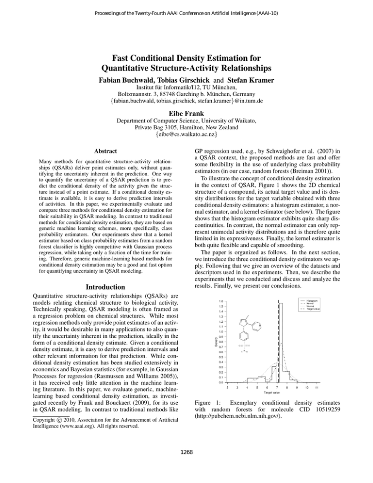
To illustrate the concept of conditional density estimation
in the context of QSAR, Figure 1 shows the 2D chemical
structure of a compound, its actual target value and its density distributions for the target variable obtained with three
conditional density estimators: a histogram estimator, a normal estimator, and a kernel estimator (see below). The figure
shows that the histogram estimator exhibits quite sharp discontinuities. In contrast, the normal estimator can only represent unimodal activity distributions and is therefore quite
limited in its expressiveness. Finally, the kernel estimator is
both quite flexible and capable of smoothing.
The paper is organized as follows. In the next section,
we introduce the three conditional density estimators we apply. Following that we give an overview of the datasets and
descriptors used in the experiments. Then, we describe the
experiments that we conducted and discuss and analyze the
results. Finally, we present our conclusions.
Many methods for quantitative structure-activity relationships (QSARs) deliver point estimates only, without quantifying the uncertainty inherent in the prediction. One way
to quantify the uncertainy of a QSAR prediction is to predict the conditional density of the activity given the structure instead of a point estimate. If a conditional density estimate is available, it is easy to derive prediction intervals
of activities. In this paper, we experimentally evaluate and
compare three methods for conditional density estimation for
their suitability in QSAR modeling. In contrast to traditional
methods for conditional density estimation, they are based on
generic machine learning schemes, more specifically, class
probability estimators. Our experiments show that a kernel
estimator based on class probability estimates from a random
forest classifier is highly competitive with Gaussian process
regression, while taking only a fraction of the time for training. Therefore, generic machine-learning based methods for
conditional density estimation may be a good and fast option
for quantifying uncertainty in QSAR modeling.
Introduction
Quantitative structure-activity relationships (QSARs) are
models relating chemical structure to biological activity.
Technically speaking, QSAR modeling is often framed as
a regression problem on chemical structures. While most
regression methods only provide point estimates of an activity, it would be desirable in many applications to also quantify the uncertainty inherent in the prediction, ideally in the
form of a conditional density estimate. Given a conditional
density estimate, it is easy to derive prediction intervals and
other relevant information for that prediction. While conditional density estimation has been studied extensively in
economics and Bayesian statistics (for example, in Gaussian
Processes for regression (Rasmussen and Williams 2005)),
it has received only little attention in the machine learning literature. In this paper, we evaluate generic, machinelearning based conditional density estimation, as investigated recently by Frank and Bouckaert (2009), for its use
in QSAR modeling. In contrast to traditional methods like
Figure 1:
Exemplary conditional density estimates
with random forests for molecule CID 10519259
(http://pubchem.ncbi.nlm.nih.gov/).
c 2010, Association for the Advancement of Artificial
Copyright Intelligence (www.aaai.org). All rights reserved.
1268
Conditional Density Estimation via Class
Probability Estimation
The normal estimator is suitable when the data is approximately normally distributed. If this is not the case, it is not
able to model the data correctly due to its inflexibility. A
popular non-parametric alternative that is also able to model
smooth, but additionally able to model multi-modal distributions is the kernel density estimator.
Before we present the three conditional density estimators
applied in our experiments we have to make some assumptions that are necessary to work with them. First, we assume that the continuous range of values of the target variable is transformed into bins by applying equal-frequency
discretization. The binning can be seen as a transformation from a regression to a classification problem. To solve
this problem we assume that we have a method that provides
class probability estimates p(c|X) for each class value c and
an instance described by attribute values X. In this way we
can obtain a weight w for each instance in the training data,
conditioned on X. These weights are then used in a standard univariate density estimator (e.g. a normal estimator)
to obtain a conditional density estimate f (y|X).
A weight w(yi |X) for a particular target value yi given an
instance X is computed by “spreading” the predicted class
probability for bin cyi that contains yi across all ncyi target
values in that bin. Formally it is given by:
w(yi |X) = n
Kernel Density Estimator In kernel density estimation
an instance from the training dataset is represented with a
Gaussian kernel (distribution). The mean of this Gaussian
distribution is the target value of the training instance; its
variance, called the kernel bandwidth σkernel , determines
how closely the estimator fits the (weighted) data points.
A small kernel bandwidth can lead to undersmoothing, and
a large σkernel to oversmoothing. In our experiments we
used the following data-dependent value based on the global
(weighted) standard deviation and the number of data points:
X
. Formally, the kernel density estimator is
σkernel = nσ1/4
given by:
Pn
2
)
fkernel (y|X) = n1 i=0 w(yi |X)N (yi , σKernel
In the remaining part of the paper we evaluate these three
conditional density estimators using QSAR datasets.
p(cyi |X)
ncyi
where n is the total number of target values in the training
data and nc is the number of target values in bin c. Intuitively the weight w(yi |X) can be seen as an estimate of
how likely it is that a future observed target value associated
with attribute values X will be close to yi , based on the class
probability estimation model that has been inferred from the
discretized training data. In the following we will present
three conditional density estimators that are based on these
weights.
Datasets and Descriptors
In this section we describe the datasets that we used in our
study. Furthermore, we present an overview of the structural and physicochemical descriptors used for encoding the
molecules.
Datasets
For our experiments we chose eight well-known publicly
available QSAR datasets from the cheminformatics web
repository1.
Histogram Density Estimator The histogram-based estimator is probably the most obvious univariate density estimator in this context since it is based on the bins provided by
the discretization. In each bin the density is assumed to be
constant and based on the bin’s width rc and the class probability or weighted target value assigned to it. The histogram
estimator can be written as follows:
Pn
I(c =cy )
fbins (y|X) = n1 i=1 w(yi |X) yi
rc
Sutherland
For the BZR (benzodiazepine receptor ligands), COX2
(cyclooxygenase-2 inhibition) and DHFR (dihydrofolate
reductase inhibitors) datasets (Sutherland, O’Brien, and
Weaver 2003) the target variable is the logarithm of the half
maximal inhibitory concentration (pIC50 = −log (IC50 )).
This quantitative measure is commonly used in pharmacology and indicates how much of a given substance is needed
to block a biological activity by half. We had to remove a
number of instances, which were considered to be inactive
in the original publication and marked with default values.
y
where I(a) is set to 1 if the proposition a is true and 0 otherwise. Note that with this estimator potentially valuable information about the relative position of y with respect to the
individual yi in a bin is discarded and that no smoothing is
performed, meaning that there can be sharp discontinuities
at the interval borders.
ER This dataset (Sutherland, O’Brien, and Weaver 2004)
lists measurements of relative binding affinities (RBA) of
compounds to the estrogen receptor with respect to βestradiol. We removed all inactive compounds from the
dataset. Since it is based on substance concentrations, we
again used its logarithm as a more meaningful target value.
Normal Density Estimator A simple estimator is the
standard univariate normal estimator:
2
fnormal (y|X) = N (µX , σX
)
with mean µX and variance σX that are both computed
based on weighted target values. The mean is defined as
Pn
µX = n1 i=0 w(yi |X)yi
CPDB The two CPDB datasets for mouse and rat data
are generated from data obtained by the carcinogenic potency project.2 The compounds’ carcinogenicity is rated
and the variance as
2
σX
=
1
n
Pn
1
2
2
i=0 w(yi |X)(yi − µX )
1269
http://www.cheminformatics.org
http://potency.berkeley.edu/chemicalsummary.html
Short-hand
BZR
COX2
DHF R
ER
CP DB mouse
CP DB rat
EP AF HM
F DAM DD
n
333
414
673
410
444
580
580
1216
Endpoint
pIC50
pIC50
pIC50
log10 (RBA)
molar TD50
molar TD50
log10 (LC50 mg)
log10 (Dose MRDD mg)
obtained a chemical description in the form of a pharmacophoric (binary) fingerprint containing more than 50 chemical descriptors. For each instance, the existence of single
atoms, functional subgroups or stereochemical descriptors
was tested. Additionally, we computed combinations of the
JOELib2 descriptors with the free tree descriptors to assess
if this leads to a gain in performance.
The JOELib2 fingerprints contain some bits for substructure occurrences and are enriched with physicochemical
properties of the molecule so we expect them to perform
better than the cFTs which encode solely substructural descriptors. However, we expect the descriptor combinations
to further enhance performance, as the JOELib2 substructural descriptors are not sufficient to capture all structural
information of a molecule.
Table 1: Overview of the datasets used for assessing our
methods. n denotes the number of compounds in the respective dataset.
according to the TD50 value, a numerical measure of the
carcinogenic potency. Based on a suggestion by the authors, we transformed
TD50 values to molar val the listed
MW , where MW is the molecular
ues: TDm
=
log
10 TD
50
50
weight. The two datasets contained several instances where
the actual structure of the compound was missing. If the
molecule could be identified uniquely via the given CAS
number, we downloaded the structure from the NCBI PubChem database3 . If this was not possible, the molecule was
removed from the set.
Experiments
We empirically compare the performance of the conditional
density estimators described above using the methodology
introduced in Frank and Bouckaert (2009). The experiments were conducted with the WEKA workbench (Hall et
al. 2009). All results are obtained using 10-times 10-fold
cross-validation. To test for significant differences, the corrected resampled paired t-test (Nadeau and Bengio 2003) is
used at a 95% significance level.
Results are discussed using random forests as the underlying class probability estimators. We used the WEKA implementation of random forests and chose an ensemble size
of 100 trees. To eliminate bias in the probability estimates,
each tree was grown from 66% of the training data, sampled
without replacement, and the remaining data was used to estimate the class probabilities at the leaf nodes. We obtained
qualitatively similar results with linear SVMs. Since we
have to deal with a discretized regression problem that is actually an ordinal classification problem, we applied WEKA’s
ordinal class classifier (Frank and Hall 2001) to exploit the
ordering information in the discretized target variable (we
use 10 bins) by creating multiple two-class problems, with
the smoothing method from Schapire et al. (2002). For each
of these binary classification problems class probability estimates were produced using random forests.
Mean entropy gain (MEG) The average log-likelihood
represents one method to measure the performance of a conditional density estimator. This measure is made more informative by subtracting the log-likelihood obtained for an
unconditional kernel density estimator, also called prior kernel, that is generated by applying a kernel density estimator
to the unweighted target values. Formally the mean entropy
gain is given by:
Pntest
log2 (f (yi |X)) − log2 (fprior (yi ))
M EG = i=0
,
ntest
where yi is the actual target value of the test instance and
ntest is the number of test instances. The desired outcome, a
positive value, means that the conditional estimator manages
to improve on the prior estimator. Note that in the context
of the histogram estimator we perform some smoothing to
avoid density values that are zero, see Frank and Hall (2001)
for details.
EPAFHM The EPAFHM (Russom et al. 1997) dataset
was generated for the purpose of developing an expert system to predict acute toxicity from chemical structure. For
our conditional density estimates we took the logarithm of
the LC50 values.
FDAMDD The FDAMDD dataset (Matthews et al. 2004)
was generated in order to predict the Maximum Recommended Daily Dose (MRDD) for pharmaceutical substances. Again, as for the EPAFHM dataset, we took the
logarithm of the target values.
A brief overview of the datasets is given in Table 1. All
datasets are available on the web4 .
Descriptors
For this paper we used three different sets of descriptors:
closed free trees (cFTs), chemical descriptors (JOE) and a
combination of both (cFTs + JOE). Firstly, we generated
substructural descriptors with the Free Tree Miner software
(FTM)(Rückert and Kramer 2004). More precisely, the
generated substructures are frequently occurring unrooted
trees. The frequency threshold was set individually for each
dataset so that approximately 1000 free trees were found.
The resulting set was further reduced to the set of closed
trees, i.e., trees occurring in the same set of structures as
one of the supertrees were removed. The occurrence of the
substructures was encoded in binary fingerprints. Secondly,
we used chemical descriptors computed with the cheminformatics library JOELib25 to represent the molecules. We
3
http://pubchem.ncbi.nlm.nih.gov/
http://wwwkramer.in.tum.de/research/machine learning/fcde
5
http://www-ra.informatik.uni-tuebingen.de/software/joelib
4
1270
Coverage and relative width In practical applications,
conditional density estimation is often used to obtain prediction intervals. Thus, it makes sense to evaluate the quality of the prediction intervals obtained from these density
estimates. To this end, we use two quality measures, the
empirical coverage of target values in the test data as well
as the average width of the predicted intervals. The goal is
to obtain narrow intervals with empirical coverage close to
the chosen confidence level. For the results shown here, a
95% confidence level was chosen. Empirical coverage is expressed as the average percentage of target values in the test
data that were in the range of the predicted intervals Ji :
Pntest
δiJi
1 if yi ∈ Ji
EmpCov = i=0
·100, with δiJi =
0 else
ntest
Figure 2: Distribution of the target values for two representative datasets.
than the kernel estimator, indicating that additional flexibility can be important.
In the next step we compare the three different descriptor
sets. The performance is somewhat inconsistent. For the histogram estimator the JOELib2 descriptors are in most cases
significantly better than the descriptor combination sets, indicating that this estimator is not able to deal with large
amounts of descriptors (overfitting). However, for the kernel, but also for the normal estimator, a dominance of the
closed free trees combined with JOELib2 descriptors is visible. The kernel estimator seems to be the better choice compared to the normal estimator for the combined descriptor
groups. For the kernel and normal estimator, it can be stated
that the combination of descriptor groups works, for most
datasets, better than single descriptor groups.
Increasing the number of discretization bins from 10 to
20 leads to a significant degradation for the histogram estimator, but for the normal and kernel estimator the effect is
relatively small in most cases and significant differences are
never observable (results not shown here).
Interval width is expressed relative to the full range of target
values in the training dataset. For instance, a relative width
of 100 means that the total interval width is equal to the full
range of target values in the training data, yielding no useful
information. We define relative width as follows:
Pntest Pm
i=0
j=0 (bij+1 − bij )
RelW id =
· 100,
ntest · (max(Ytrain ) − min(Ytrain ))
where bij+1 and bij are the interval borders (the histogram
and kernel estimators can produce multiple intervals) and
Ytrain is the set of training target values.
Results
The following section evaluates the experimental results and
is structured as follows. In the first part the three conditional
density estimators are compared with respect to the mean
entropy gain and the best descriptor set is determined. In
the second part we will analyze the coverage and the size of
the predicted intervals. In the third part the performance of
GP regression is compared to that of the conditional density
estimators described above.
Results for Prediction Intervals
To evaluate the prediction intervals, we use the two quality
measures from above, the empirical coverage of target values in the test data as well as the relative width of the predicted intervals. The aim is to obtain narrow intervals with
empirical coverage close to the chosen confidence level. For
the results shown here a 95% confidence level was chosen.
All results (Table 3) are calculated with random forests
with cFTs+JOE descriptors and are evaluated by coverage
and relative width. The remaining results are omitted due to
lack of space. Furthermore, we present only the results for
10 discretization intervals. Results for 20 intervals yield a
comparable relative performance for the kernel and the normal estimator.
The results show that the kernel as well as the normal estimator always produces a significantly higher coverage than
the histogram estimator. Both show in all cases a coverage
that is often above or near the confidence interval of 95%.
This is the desired outcome, which is important for practical
applications where the end user expects reliable prediction
intervals. The strong performance of the kernel and normal
estimator is contrasted by the failure of the histogram esti-
Descriptor Analysis and Results for Mean Entropy
Gain
The main goal of this first evaluation section is to compare
the different conditional density estimators on different feature sets and also to find out which descriptor set is working
best. In the result table (Table 2a), the statistical significance
is measured with respect to the kernel estimator.
The results show that the kernel estimator improves in a
statistically significant way over the histogram estimator in
all cases. In fact, the latter is outperformed by the prior
estimator in nearly all cases. Although the normal estimator is not flexible (because it is only able to model an
unimodal Gaussian distribution), it also performs well compared to the histogram estimator. In this context it is illustrative to consider the distribution of measured values (Figure
2). Most datasets show roughly a normal distribution (sometimes skewed or with a tendency towards a multimodal distribution (ER)). In comparison to the kernel estimator, there
are statistically significant differences in about 50% of the
cases. The normal estimator performs equally well or worse
1271
Dataset
BZR cFTs
BZR JOE
BZR comb.
COX2 cFTs
COX2 JOE
COX2 comb.
DHFR cFTs
DHFR JOE
DHFR comb.
ER cFTs
ER JOE
ER comb.
CPDB mouse cFTs
CPDB mouse JOE
CPDB mouse comb.
CPDB rat cFTs
CPDB rat JOE
CPDB rat comb.
EPAFHM cFTs
EPAFHM JOE
EPAFHM comb.
FDAMDD cFTs
FDAMDD JOE
FDAMDD comb.
RF Kernel
RF Hist.
RF Normal
0.27± 0.22
-0.71± 0.49 •
0.27± 0.18
0.41± 0.14
−0.31±0.40 •
0.28± 0.13
0.45±0.17
-0.39± 0.43 •
0.34±0.14
0.36± 0.22
-0.19± 0.41 •
0.17± 0.27
0.56± 0.12
0.05±0.34 •
0.35± 0.10
0.58±0.15
-0.03± 0.37 •
0.37±0.14
0.53± 0.21
-0.70± 0.47 •
0.76±0.30
0.56± 0.30
−0.16±0.34 •
0.57± 0.25
0.65±0.21
-0.17± 0.32 •
0.72± 0.27
0.30± 0.26
-0.65± 0.57 •
0.41± 0.19
0.65±0.17
0.09±0.36 •
0.51± 0.10
0.61± 0.20
-0.07± 0.41 •
0.56±0.13
0.13± 0.22
-1.11± 0.55 •
0.24± 0.15
0.19± 0.10
−0.54±0.37 •
0.21± 0.19
0.25±0.16
-0.58± 0.43 •
0.26±0.16
0.28± 0.15
-0.73± 0.41 •
0.33± 0.11
0.24± 0.09
-0.37± 0.28 •
0.22± 0.07
0.35±0.11
−0.33±0.33 •
0.34±0.08
0.47± 0.15
-0.57± 0.42 •
0.49± 0.12
0.69±0.15
0.11±0.36 •
0.60±0.13
0.68± 0.14
0.05± 0.34 •
0.59± 0.12
0.49± 0.11
-0.32± 0.29 •
0.37±0.08
0.43± 0.08
−0.02±0.19 •
0.27± 0.07
0.52±0.09
-0.07± 0.24 •
0.35± 0.07
◦, • statistically significant improvement or degradation
•
•
•
•
•
◦
•
•
•
•
•
•
GPR
0.15± 0.18
0.18± 0.16
0.23±0.20
0.24± 0.18
0.40±0.14
0.38± 0.15
0.74± 0.27
0.67± 0.30
0.79±0.27
0.39± 0.14
0.52± 0.21
0.70±0.19
0.14± 0.21
0.20±0.25
0.20±0.20
0.28± 0.16
0.25± 0.15
0.30±0.14
0.54± 0.18
0.64± 0.25
0.75±0.26
0.27± 0.09
0.27± 0.09
0.28±0.12
(a)
•
•
•
•
◦
•
•
•
Dataset
RF
GPR
BZR cFTs
7.49±0.20
301.32± 37.20
2.80±0.04
200.10± 18.70
BZR JOE
BZR comb.
6.45±0.10
372.87± 50.55
COX2 cFTs
9.54±0.26
530.62± 65.39
COX2 JOE
3.51±0.05
402.93± 33.26
8.42±0.13
628.83± 84.60
COX2 comb.
DHFR cFTs
16.76±0.32
1939.98± 181.66
5.91±0.08
1434.38± 113.72
DHFR JOE
DHFR comb.
12.85±0.16
2179.09± 224.18
ER cFTs
19.85±0.48
1890.43± 187.80
ER JOE
3.10±0.43
324.63± 53.35
14.86±0.26
2140.66± 226.27
ER comb.
CPDB mouse cFTs
18.54±0.30
1158.29± 31.15
4.24±0.06
437.31± 20.23
CPDB mouse JOE
CPDB mouse comb.
14.38±0.17
1295.11± 34.37
CPDB rat cFTs
25.50±0.41
2321.26± 57.94
CPDB rat JOE
5.45±0.08
884.70± 43.78
19.29±0.21
2532.12± 88.24
CPDB rat comb.
EPAFHM cFTs
25.94±0.40
2486.02± 97.88
4.67±0.07
932.37± 50.16
EPAFHM JOE
EPAFHM comb.
19.02±0.20
2765.35± 113.96
FDAMDD cFTs
66.96±0.93
16928.35±1486.98
FDAMDD JOE
11.50±0.18
8160.61± 666.56
FDAMDD comb.
56.15±0.77
15753.52± 707.52
◦, • statistically significant improvement or degradation
•
•
•
•
•
•
•
•
•
•
•
•
•
•
•
•
•
•
•
•
•
•
•
•
(b)
Table 2: Results with standard deviations. (a) Mean improvement in log-likelihood vs prior estimate, using random forests and
10 bins. The best feature set for a conditional density estimator and a dataset is marked in bold. (b) Training times in seconds.
Gaussian Process regression was applied with inputs normalized to [0, 1]. The target was also normalized, to make
choosing an appropriate noise level σ easier. Predictions
were transformed back into the original range of the target variable. The noise level σ for GPR, and γ for the
RBF kernel, were optimized using internal cross-validation,
based on optimizing for mean entropy gain, with values
10i with i ∈ {−5, 4, ..., 4, 5} for γ, and values 10i with
i ∈ {−2, −1.8, −1.6, ..., −0.4, −0.2, 0} for σ. To save runtime, 5-fold cross-validation was used to perform an initial complete exploration of all pairs of parameter values.
Subsequently, greedy exploration based on 10-fold crossvalidation was performed, starting with the best pair found
in the initial complete run.
mator which is unable to get close to the confidence interval
of 95%. Regarding the relative width of the prediction intervals, the histogram estimator shows narrower (better) interval widths than the kernel and/or normal estimator in three
of the eight cases. This is due to its low coverage and explained by the fact that the kernel and the normal estimator
perform smoothing.
Generally, the end user requires reliable prediction intervals, so that more emphasis should be given to coverage than
to relative width. But particular attention must be paid to
those cases where one method dominates another one based
on both criteria. For the kernel and normal estimator vs the
histogram estimator, this is the case for five of eight datasets.
The opposite is never the case. This confirms the strong performance of the kernel and normal estimators in comparison
to the histogram-based method.
Considering the relative performance of the normal and
kernel estimators for interval estimation, we can see that
they are largely competitive. The former generally exhibits
elevated coverage levels and larger intervals. There are two
cases where the former dominates the latter with respect two
both criteria (the CPDB datasets). Vice versa, there is one
dataset (COX2) where the kernel estimators performs better
according to both criteria.
We performed experiments with linear kernels and RBF
kernels. As the results using linear kernels were worse than
all other results presented here, we focus on the results for
RBF kernels. In Tables 2a and 3, the performance of Gaussian Process regression using RBF kernels is given in the
last column for each quantity (mean entropy gain, coverage
and relative width). As can be seen, the performance of GP
regression is generally on par or only slightly worse than the
one of the kernel estimator. However, looking at the running
times in Table 2b, it is clear that GP regression requires substantially more time for training (sometimes up to a factor of
100 or more), because parameter optimization is necessary
to reach competitive levels of performance.
Comparison to Gaussian Process Regression
In the following, we present our experimental comparison with Gaussian Process regression on the eight datasets.
1272
Dataset
BZR
COX2
DHFR
ER
CPDB mouse
CPDB rat
EPAFHM
FDAMDD
RF Kernel
95.79± 3.69
95.68±2.76
96.30± 2.12
95.90± 2.94
95.11± 3.56
95.83± 2.69
96.81± 2.20
96.03± 1.71
Coverage
Relative width
RF Hist.
RF Normal
GPR
RF Kernel
RF Hist.
RF Normal
85.42±6.48 •
97.93±2.32 ◦
93.70±3.82
59.92±3.05
58.85±2.58
61.70± 3.30
86.76±4.80 •
95.26± 3.14
94.13±3.37
69.82±1.93
61.00±1.94 ◦
70.69± 1.98
90.97±3.40 •
97.86±1.72 ◦
95.75±2.72
35.85±3.20
47.50± 1.67 •
35.97± 3.07
86.78±5.74 •
97.29±2.77
92.59±3.95 •
66.27±2.13
59.62± 2.12 ◦
68.59± 2.24
88.37±5.11 •
95.27±3.35
94.14±4.36
49.89±2.51
64.34± 2.55 •
48.80±2.31
90.41±3.93 •
96.60±2.36
95.17±3.21
52.32±2.14
62.34± 2.05 •
51.05± 2.06
91.97±3.54 •
97.03±2.12
94.57±3.11
51.72±2.59
58.90± 1.55 •
48.16± 2.37
89.92±2.94 •
96.76±1.42 ◦
92.26±2.35 •
46.27±0.61
56.19± 1.50 •
47.38± 0.64
◦/• statistically significant improvement/degradation; best density estimator per dataset in bold print
•
•
•
◦
◦
◦
•
GPR
66.16± 4.39
67.38± 0.94
30.35±4.09
47.45±1.41
49.99± 4.29
50.77±1.63
35.72±4.69
41.29±1.19
•
◦
◦
◦
◦
◦
Table 3: Quality of prediction intervals with standard deviations, using random forests and 10 bins and Gaussian Process
regression, with cFTs combined with JOE descriptors. Best density estimator per dataset and criterion in bold print.
Conclusion
Frank, E., and Hall, M. 2001. A simple approach to ordinal
classification. In Proc. of ECML ’01, 145–156. Springer.
Hall, M.; Frank, E.; Holmes, G.; Pfahringer, B.; Reutemann,
P.; and Witten, I., H. 2009. The WEKA data mining software: An update. SIGKDD Explorations 11(1).
Matthews, E.; Kruhlak, N.; Benz, R.; and Contrera, J. 2004.
Assessment of the health effects of chemicals in humans:
I. QSAR estimation of the maximum recommended therapeutic dose (MRTD) and no effect level (NOEL) of organic
chemicals based on clinical trial data. Current Drug Discovery Technologies 1(1):61–76.
Nadeau, C., and Bengio, Y. 2003. Inference for the generalization error. Machine Learning 52(3):239–281.
Rasmussen, C. E., and Williams, C. K. I. 2005. Gaussian Processes for Machine Learning (Adaptive Computation and Machine Learning). MIT Press.
Rückert, U., and Kramer, S. 2004. Frequent Free Tree Discovery in Graph Data. In Proc. of SAC ’04, 564–570. ACM
Press.
Russom, C.; Bradbury, S.; Broderius, D.; Hammermeister,
S.; and Drummond, R. 1997. Predicting modes of action
from chemical structure: Acute toxicity in the fathead minnow (pimephales promelas). Environmental Toxicology and
Chemistry 5(16):948–967.
Schapire, R. E.; Stone, P.; McAllester, D. A.; Littman,
M. L.; and Csirik, J. A. 2002. Modeling auction price uncertainty using boosting-based conditional density estimation.
In Proc. of ICML ’01, 546–553. Morgan Kaufmann.
Schwaighofer, A.; Schroeter, T.; Mika, S.; Laub, J.; ter Laak,
A.; Sülze, D.; Ganzer, U.; Heinrich, N.; and Müller, K.R. 2007. Accurate solubility prediction with error bars for
electrolytes: A machine learning approach. J. Chem. Inf.
Model. 47:407–424.
Sutherland, J. J.; O’Brien, L. A.; and Weaver, D. F. 2003.
Spline-fitting with a genetic algorithm: A method for developing classification structure-activity relationships. J. Chem.
Inf. Model. 43(6):1906–1915.
Sutherland, J. J.; O’Brien, L. A.; and Weaver, D. F. 2004. A
comparison of methods for modeling quantitative structureactivity relationships. J. Med. Chem. 47(22):5541–5554.
In this paper we considered methods for conditional density estimation based on generic machine learning methods,
more precisely, class probability estimators, for their use in
QSAR modeling. Our experimental results show that kernel
density estimators based on weighted target values are the
best choice for a wide range of target distributions, in particular with respect to the log-likelihood. If the target values for
the dataset are (conditionally) normally or roughly normally
distributed, the normal estimator is also a good choice. The
latter appears to work particularly well for the prediction of
intervals. The use of the histogram estimator should rather
be avoided, as its lack of smoothing generally leads to sharp
discontinuities between the bins.
We also compared with Gaussian Process (GP) regression, one of the standard methods for conditional density
estimation. GP regression with a linear kernel failed to produce competitive results, whereas GP regression with an
RBF kernel produced results on par with the best obtained
using class probability estimation with random forests. Due
to the required parameter optimization, however, the running times exceeded those of the method presented here by a
large factor. Therefore, conditional density estimation based
on class probability estimation, based on using kernel and
normal estimators in conjunction with random forests can
be seen as good options for QSAR problems. Finally, it is
interesting to note that the approach considered here can be
applied to take into account costs at prediction time as the
full conditional density could be taken into account for this
purpose.
Acknowledgements
This work was partially supported by
FP7 project (HEALTH-F5-2008-200787)
(http://www.opentox.org).
the EU
OpenTox
References
Breiman, L. 2001. Random forests. Machine Learning
45(1):5–32.
Frank, E., and Bouckaert, R. 2009. Conditional density estimation with class probability estimators. In Proc. of ACML
’09. Springer.
1273