Proceedings of the Twenty-Fifth AAAI Conference on Artificial Intelligence
Time Complexity of Iterative-Deepening A*:
The Informativeness Pathology (Abstract)
Levi Lelis
Sandra Zilles
Robert C. Holte
Computing Science Department
University of Alberta
Edmonton, AB, Canada T6G 2E8
(santanad@cs.ualberta.ca)
Computer Science Department
University of Regina
Regina, SK Canada S4S 0A2
(zilles@cs.uregina.ca)
Computing Science Department
University of Alberta
Edmonton, AB, Canada T6G 2E8
(holte@cs.ualberta.ca)
Introduction
the number of nodes expanded by emulating IDA*’s iteration using π(t |t) and β(t) to estimate the number of states
of a type at a level of search. Let N (i, t, s∗ , d) be the number of pair of states (ŝ, s) ∈ E with T ((ŝ, s)) = t, at a
level i, rooted at the start state s∗ and with a depth bound
d. CDP calculates N (i, t, s∗ , d) recursively by multiplying
N (i − 1, u, s∗ , d), π(t|u) and β(u) for all u ∈ T .
As our basic type system, Th , we use Zahavi et
al.’s basic “two-step” model, defined (in our notation)
as Th (ŝ, s) = (h(ŝ), h(s)), with (ŝ, s) ∈ E. Another “more informed” type system is Tgc (ŝ, s) =
(Th (ŝ, s), c(s, 0), . . . , c(s, H), gc(s, 0), . . . , gc(s, H)).
Where c(s, k) is the number of children of s whose h-value
is k, and H is the maximum h-value observed in the sampling process and gc(s, k) is the number of grandchildren
of s whose h-value is k.
Intuitively, if T1 is more informed than T2 one would expect predictions using T1 to be at least as accurate as the
predictions using T2 , since all the information that is being
used by T2 to condition its predictions is also being used by
T1 ((Zahavi et al. 2010), p. 59). However, our experiments
show that this is not always true. The underlying cause of
poorer predictions by T1 when T1 is more informed than T2
is the discretization effect.
Korf et al. (2001) developed a formula, KRE, to predict the
number of nodes expanded by IDA* for consistent heuristics. They proved that the predictions were exact asymptotically (in the limit of large d), and experimentally showed
that they were extremely accurate even at depths of practical interest. Zahavi et al. (2010) generalized KRE to work
with inconsistent heuristics and to account for the heuristic
values of the start states. Their formula, CDP, is intuitively
described in the next section. For a full description of CDP
the reader is referred to Zahavi et al. (2010).
Our research advances this line of research in three ways.
First, we identify a source of prediction error that has hitherto been overlooked. We call it the “discretization effect”.
Second, we disprove the intuitively appealing idea that a
“more informed” prediction system cannot make worse predictions than a “less informed” one. More informed systems are more susceptible to the discretization effect, and
in our experiments the more informed system makes poorer
predictions. Our third contribution is a method, called “truncation”, which makes a prediction system less informed,
in a carefully chosen way, so as to improve its predictions
by reducing the discretization effect. In our experiments truncation improved predictions substantially.
The -Truncation Prediction Method
The CDP Prediction Framework
Consider the problem of predicting the outcome of flipping
a biased coin that yields tails in 90% of all trials, modeled in
the CDP framework. An initial type init generates either type
tails or type heads, where p(tails|init) = 0.9, p(heads|init) =
0.1 and binit = 1. Suppose π and β(init) approximates respectively p and binit exactly and N (i, init, s∗ , d) = 1. Then
CDP would predict that 0.9 tails and 0.1 heads will occur
at level i + 1. However, a prediction of 1.0 tails and 0.0
heads occurring at level i + 1 has a smaller expected absolute error when compared to CDP’s prediction. We call this
phenonemon (better predictions arising when less accurate
probability estimates are used) the discretization effect.
If a type t is generated with low probability from a type
t and if N (i, t, s∗ , d) is small, it may be possible to reduce
expected absolute error by disregarding t , i.e., by artificially
setting π(t |t) to zero at level i of the prediction calculation.
Our approach, which we call -truncation, avoids the discretization effect and can be summarized as follows.
Let S be the set of states, E ⊆ S × S the set of (directed)
edges over S representing the parent-child relation in the
underlying state space.
Definition 1 T = {t1 , . . . , tn } is a type system for (S, E)
if it is a disjoint partitioning of E. For every (ŝ, s) ∈ E,
T (ŝ, s) denotes the unique t ∈ T with (ŝ, s) ∈ t. For all
t, t ∈ T , p(t |t) denotes the probability that a node s with
parent ŝ such that T (ŝ, s) = t generates a node c such that
T (s, c) = t . Finally, bt denotes the average number of
nodes c generated from a parent s and grandparent ŝ with
T (ŝ, s) = t.
CDP samples the state space in order to estimate p(t |t)
and bt for all t, t ∈ T . We denote by π(t |t) and β(t) the
respective estimates thus obtained. Intuitively, CDP predicts
Copyright © 2011, Association for the Advancement of Artificial
Intelligence (www.aaai.org). All rights reserved.
1800
1. As before, sample the state space to obtain π(t|u).
Signed Error
d
2. Compute a cutoff value i for each i between 1 and d.
IDA*
Th,b
Tgc
Absolute Error
-Tgc
Th,b
Tgc
-Tgc
8-puzzle. Inconsistent Heuristic. r=1
3. Use i to define π i (t|u), a version of π(t|u) that is specific
to level i. In particular, if π(t|u) < i then π i (t|u) = 0;
the other π i (t|u) are set by scaling up the corresponding
π(t|u) values so that they sum to 1.
24
135.7
1.03
1.45
0.93
0.47
0.66
0.37
25
226.7
1.04
1.52
0.98
0.42
0.65
0.34
4. In computing CDP use π i (t|u) at level i instead of π(t|u).
52
28,308,808.8
1.25
1.28
1.14
0.14
0.17
0.09
53
45,086,452.6
1.23
1.29
1.13
0.16
0.20
0.11
22
58.5
1.00
1.34
0.96
0.47
0.62
0.41
23
95.4
1.01
1.39
0.98
0.45
0.62
0.38
15-puzzle. Manhattan Distance. r=25
The calculation of the i values requires computing CDP
predictions for a set of start states and, for each level i in
each of these prediction calculations, solving a set of small
linear programs that minimizes the expected error. The solutions of the linear programs suggest an i (details are omitted
due to lack of space).
54
85,024,463.5
1.36
1.41
1.22
0.21
0.27
0.15
55
123,478,361.5
1.36
1.45
1.24
0.24
0.31
0.17
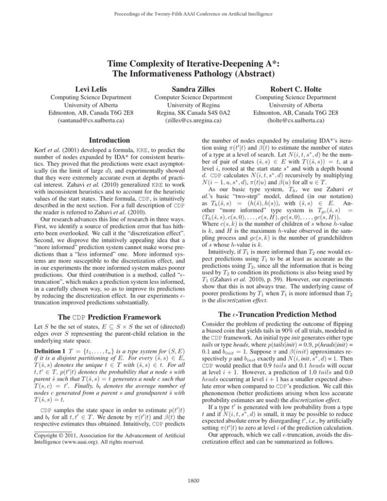
Table 1: Informativeness Pathology
Th,b (s, s ) = (Th , blank(s), blank(s )) where blank(s) returns the kind of location (corner, edge, or middle) the blank
occupies in state s. Tgc,b is defined analogously. For square
versions of the puzzle Tgc is exactly the same as Tgc,b and
therefore Tgc is more informed than Th,b .
The inconsistent heuristic we used for the 8-puzzle is the
one defined by Zahavi et al. (2010). Two PDBs were built,
one based on tiles 1-4, and one based on tiles 5-8. The first
PDB is consulted for states having the blank in an even location and the second PDB is consulted otherwise. The results,
with r=1, are shown at the top of Table 1. Here we see the
informativeness pathology: Tgc ’s predictions are worse than
Th,b ’s, despite its being a refinement of Th,b . Applying truncation substantially reduces Tgc ’s prediction error.
For the 15-puzzle, we used 1,000 random start states to
measure prediction accuracy. To define π(t|u) and βt , one
billion random states were sampled and, in addition, we used
the process described by Zahavi et al. (2010): we sampled
the child of a sampled state if the type of that child had not
yet been sampled. The bottom of Table 1 gives the results
when Manhattan Distance is the heuristic, Th,b and Tgc are
the type systems and r=25. Here again we see the pathology
(Th,b ’s predictions are better than Tgc ’s) which is eliminated
by -truncation. Our method also improved considerably the
prediction accuracy for the 10 and 15 pancake puzzles (results omitted due to lack of space).
Experiments and Conclusion
Our experiments shows that, 1) more informed type systems can produce poorer predictions and, 2) the -trucantion
method improves the predictions of a more informed type
system and prevents the pathology from occurring.
The choice of the set of start states is the same used by
Zahavi et al. (2010): start state s is included in the experiment with depth bound d only if IDA* would actually have
used d as a depth bound in its search with s as the start state.
Unlike an actual IDA* run, we count the number of nodes
expanded in the entire iteration for a start state even if the
goal is encountered during the iteration.
For each prediction system we will report the ratio of the
predicted number of nodes expanded, averaged over all the
start states, to the actual number of nodes expanded, on average, by IDA*. This ratio will be rounded to two decimal places and it is called the (average) signed error. The
signed error is the same as the “Ratio” reported by Zahavi et
al. (2010) and is appropriate when one is interested in predicting the total number of nodes that will be expanded in
solving a set of start states. It is not appropriate for measuring the accuracy of the predictions on individual start states
because errors with a positive sign cancel errors with a negative sign. To evaluate the accuracy of individual predictions, the appropriate measure is absolute error. For each
instance one computes the absolute value of the difference
between the predicted and the actual number of nodes expanded, divide this difference by the actual number of nodes
expanded, adds these up over all start states, and divides by
the total number of start states. A perfect score according to
this measure is 0.0.
Zahavi et al. (2010) introduced a method for improving
predictions for single start states. Instead of directly predicting how many nodes will be expanded for depth bound d
and start state s, all states, Sr , at depth r < d are enumerated
and one then predicts how many nodes will be expanded for
depth bound d − r when Sr is the set of start states. We applied this technique in our experiments. The value of r for
each experiment is specified below.
We ran experiments on the 8 and 15 sliding tile puzzles and used the same type system as Zahavi et al. (2010),
which is a refinement of Th we call Th,b . Th,b is defined by
Acknowledgements
This work was supported by the Laboratory for Computational Discovery at the University of Regina. The authors gratefully acknowledge the research support provided
by Alberta’s Informatics Circle of Research Excellence
(iCORE), the Alberta Ingenuity Centre for Machine Learning (AICML), and Canada’s Natural Sciences and Engineering Research Council (NSERC).
References
R. E. Korf, M. Reid, and S. Edelkamp. Time complexity of
iterative-deepening-A∗ . Artif. Intell, 129(1-2), 2001.
U. Zahavi, A. Felner, N. Burch, and R. C. Holte. Predicting
the performance of ida* using conditional distributions. J.
Artif. Intell. Res. (JAIR), 37:41–83, 2010.
1801