Proceedings of the Twenty-Sixth AAAI Conference on Artificial Intelligence
Investigating the Effectiveness of Laplacian-Based Kernels in Hub Reduction
Ikumi Suzuki
Kazuo Hara
Nara Institute of Science& Technology
Ikoma, Nara - Japan
ikumi-s@is.naist.jp
National Institute of Genetics
Mishima, Shizuoka - Japan
kazuo.hara@gmail.com
Masashi Shimbo
Yuji Matsumoto
Nara Institute of Science& Technology Nara Institute of Science& Technology
Ikoma, Nara - Japan
Ikoma, Nara - Japan
matsu@is.naist.jp
shimbo@is.naist.jp
Abstract
Marco Saerens
Université Catholique de Louvain
Louvain-la-Neuve - Belgium
marco.saerens@uclouvain.be
are known. If test objects follow the same distribution as
that of the objects in the dataset, hubs in the dataset should
frequently appear in the knn list for test objects as well. As
a result, hub objects pose strong bias on the predicted labels, causing the classification results to be inaccurate. As
we will discuss in a later section, hubs also impair information retrieval, and the label propagation methods for semisupervised classification.
In this paper, we examine if Laplacian-based kernels, such
as the commute-time kernels (Saerens et al. 2004) and
the regularized Laplacian (Chebotarev and Shamis 1997;
Smola and Kondor 2003), are effective for reducing hubs.
We explore Laplacian-based kernels based on our observation that in the implicit feature space, the inner product with
the centroid is uniform for all objects in the dataset; thus, no
objects are closer to the centroid. According to Radovanović
et al., objects close to the centroid become hubs, and we
expect these kernels are more robust to the hubness phenomenon. We empirically examine if Laplacian-based kernels reduce hubs and consequently improve the performance
of information retrieval as well as multi-class and multilabel k-nearest neighbor classification.
A “hub” is an object closely surrounded by, or very similar to, many other objects in the dataset. Recent studies by
Radovanović et al. indicate that in high dimensional spaces,
hubs almost always emerge, and objects close to the data centroid tend to become hubs. In this paper, we show that the
family of kernels based on the graph Laplacian makes all objects in the dataset equally similar to the centroid, and thus
they are expected to make less hubs when used as a similarity
measure. We investigate this hypothesis using both synthetic
and real-world data. It turns out that these kernels suppress
hubs in some cases but not always, and the results seem to be
affected by the size of the data. However, for the datasets in
which hubs are indeed reduced by the Laplacian-based kernels, these kernels work well in ranking and classification
tasks. This result suggests that the amount of hubs, which
can be readily computed in an unsupervised fashion, can be
a yardstick of whether Laplacian-based kernels work effectively for a given data.
Introduction
In recent studies, Radovanović et al. investigated hubs that
emerge in high dimensional space (Radovanović, Nanopoulos, and Ivanović 2010a; 2010b). A hub is an object similar
(or close) to many other objects in a dataset. Radovanović
et al. observed that hub objects emerge as dimension increases, for a number of common similarity or distance measures. They also made a notable finding that the objects
closer (more similar) to the data mean, or centroid, tend to
become hubs.
Hub objects emerge even in space of moderately high
dimension (e.g., 50-dimensions), whereas systems for real
data analysis, such as those for natural language processing,
often deal with more than one million features (dimensions).
As Radovanović et al. have pointed out, hubs impair the
accuracy of k-nearest neighbor (knn) classification. In knn
classification, the label of a test object is predicted by the
(weighted) majority voting of the knn objects whose labels
Laplacian-based Kernels for Graph Vertices
We first present a brief review of Laplacian-based kernels.
Let G be an undirected graph with n vertices, and let A
be its adjacency matrix. The edges of G may have positive
weights representing the degree of similarity between vertices. In this case, A is an affinity matrix holding the edge
weights as its components. The (combinatorial) Laplacian
L of G is an n × n matrix defined as
L = D − A,
(1)
where D is a diagonal matrix with diagonals [D]ii = ∑ j [A]i j .
L is positive semidefinite and has n orthogonal eigenvectors
ui and n corresponding eigenvalues λi . We assume that the
indices for eigenvalues/eigenvectors are arranged in ascending order of eigenvalues, λ1 ≤ λ2 ≤ · · · ≤ λn . A well-known
property of L is that λ1 = 0 and u1 = 1 (a vector of all 1’s).
c 2012, Association for the Advancement of Artificial
Copyright Intelligence (www.aaai.org). All rights reserved.
1112
Laplacian-based Kernels
which list objects similar (or near) to a query object according to a certain similarity (or distance) measure. Because
hub objects are similar to many other objects in the dataset,
they appear in the nearest neighbor lists of those many objects, Thus, search results become less meaningful, as the
same objects (hubs) are included in the search results irrespective of the query. And Radovanović et al. found that
hubs nearly always appear in high dimensional data.
Applications affected by hubs include information retrieval and k-nearest neighbor classification. Graph-based
semi-supervised classification methods, such as label propagation (Zhu, Ghahramani, and Lafferty 2003; Zhou et al.
2004), may also be affected, as these methods are typically
run on k-nearest neighbor graphs.
Whether or not hubs exist in a dataset can be checked by
counting the number of times that each object x appears in
the k-nearest neighbor list of other objects. Let this number
be Nk (x). If hubs exist in the dataset, the distribution of Nk
should skew to the right (provided that k n, where n is the
number of the objects).
In a manner similar to (Radovanović, Nanopoulos, and
Ivanović 2010a), we illustrate the emergence of hubs using
synthetic data consisting of 500 objects, each of which is a
d-dimensional binary vector. To generate this data set, we
first sample, for each dimension i = 1, . . . , d, a real number
from the log-normal distribution with mean 5 and variance
1, and compute its rounded integer ni . We then choose ni
objects (vectors) out of 500 uniformly at random, and assign
1 to their ith component. After 500 d-dimensional binary
vectors are generated in this way, we measure their pairwise
similarity by the cosine of the angle between them.
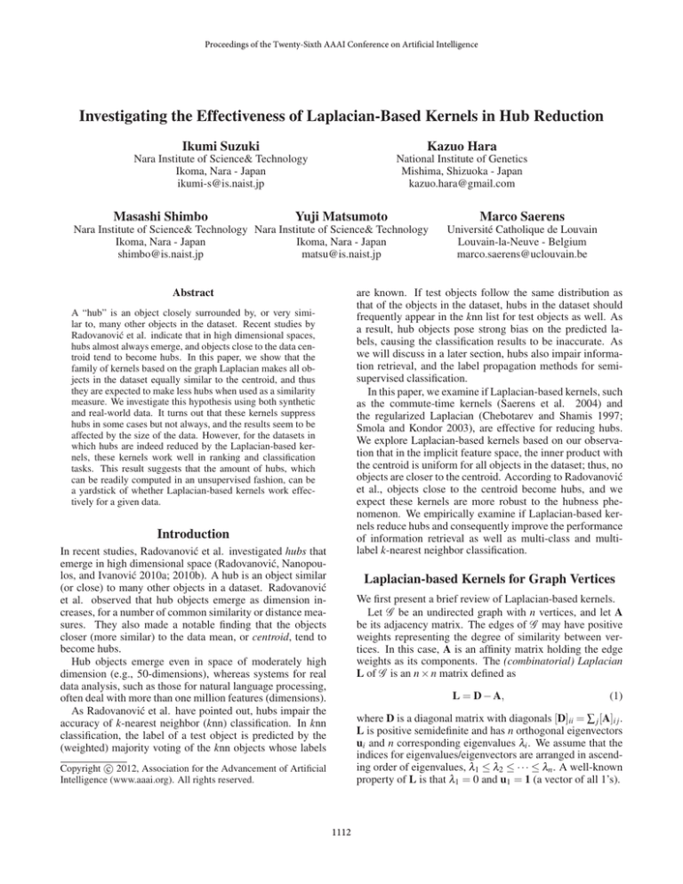
The histograms of N10 frequency for two datasets with
different dimensions d (d = 10, 50) are shown in the top panels of Figure 1. We can see objects with extremely large N10
values (e.g., the point at N10 = 60) in the top right panel
(50-dimensional data), while no such points can be seen for
10-dimensional data.
Another important finding by Radovanović et al. is that
in high dimensional spaces, objects similar (or close) to the
data mean (centroid) tend to become hubs. We can verify this with the dataset of 50-dimensional vectors above.
The bottom panels of Figure 1 are the scatter plots of N10
values of the data objects against their cosine similarity to
the centroid. For d = 50 (high-dimensional data; bottomright), N10 values show a strong correlation with the similarity to the centroid, whereas for d = 10 (low-dimensional
data; bottom-left), the correlation is much weaker.
In machine learning community, graph Laplacian has been
used as the building block of various kernels defining inner
products between vertices. Below are the most popular of
such Laplacian-based kernels.
Commute-time kernels (Saerens et al. 2004)
LCT = L+
(pseudo-inverse of L),
(2)
Regularized Laplacian (Chebotarev and Shamis 1997;
Smola and Kondor 2003)
LRL = (I + β L)−1 ,
(3)
Diffusion kernels (Kondor and Lafferty 2002)
LDF = exp(−β L),
(4)
where β (≥ 0) is a parameter of the regularized Laplacian
and the diffusion kernels. Note that while we do not discuss
them in this paper, variations of these kernels exist which
use the normalized Laplacian L = D−1/2 LD−1/2 (Chung
1997) in place of L in their definition.
The above kernels can be interpreted as transformations of
Laplacian L through eigenvalue regularization (Smola and
Kondor 2003). To be precise, all the Laplacian-based kernels above (henceforth denoted by K) can be decomposed
as follows, using n pairs of eigenvalues and eigenvectors
{(λi , ui )} (i = 1, . . . , n) of L.
n
K = ∑ r(λi )ui uTi ,
(5)
i=1
where r : [0, ∞) → [0, ∞) is a regularization operator, which
characterizes each Laplacian-based kernel. For the three
kernels above,
0,
λ = 0;
Commute-time kernels r(λ ) =
1/λ λ 6= 0,
Regularized Laplacian r(λ ) = 1/(1 + β λ ),
Diffusion kernels r(λ ) = exp(−β λ ).
As Eq. (5) shows, Laplacian-based kernels have the same
eigenvectors as Laplacian L. Their eigenvalues, on the other
hand, are transformed by function r(λ ). To suppress the
contribution of large λ ’s which represent high-frequency
components, r(λ ) is in general a non-increasing function for
λ > 0.
In the rest of the paper, we focus on the commute-time
kernels LCT and the regularized Laplacian LRL . Diffusion
kernels LDF show properties similar to LRL .
Hubs in High Dimensional Space
Hubness Phenomenon and Laplacian-based
Kernels
High dimensionality causes various problems that go under
the name of curse of dimensionality. The most well-known
“curse” includes overfitting (Hastie, Tibshirani, and Friedman 2001; Bishop 2006) and distance concentration (Beyer
et al. 1999; François, Wertz, and Verleysen 2007).
The “emergence of hubs” is a new type of the curse which
has been discovered only recently (Radovanović, Nanopoulos, and Ivanović 2010a). This phenomenon particularly affects methods based on nearest neighbor search, i.e., those
If objects close to the data centroid tend to become hubs,
a possible direction to their reduction should be to seek
a similarity (or distance) measure which evaluates all objects equally similar to (or distant from) the centroid. We
show that the Laplacian-based kernels indeed give measures
which meet this requirement.
1113
Laplacian-based kernels and similarity to the
centroid
We now restrict K to Laplacian-based kernels, i.e., those
which can be expressed as in Eq. (5). We show that these
kernels define similarity measures which make the data centroid equally similar to all objects in the dataset.
Because Laplacian-based kernels assume that the data is
represented as a graph, we treat the vector dataset X as a
fully-connected graph. In this graph, data objects xi corresponds to vertices, and edge weights are given by the pairwise similarity of objects measured in the original vector
space D.1 In other words, the weighted adjacency matrix A
of this fully-connected graph is given by the all-pairs similarity matrix for the dataset computed in D. There may be
many ways to measure similarity, but we only require that
the similarity score given by A be non-negative and symmetric; hence [A]i j = [A] ji ≥ 0 for all i, j. Given such an A,
we compute the graph Laplacian and then a Laplacian-based
kernel matrix K, e.g., using one of Eqs. (2)–(4).
Now, recall that the Laplacian-based kernels share the
same eigenvectors as the Laplacian L from which they are
computed, but the eigenvalues are transformed by r(·); see
Eq. (5). In particular, for the smallest eigenvalue λ1 of L
and its corresponding eigenvector u1 , it holds that Ku1 =
r(λ1 )u1 . And since u1 = 1 and λ1 = 0, we have
Figure 1: Top panels: Histograms of N10 frequency for two
synthetic datasets in low (d = 10) and high (d = 50) dimensional feature spaces. Bottom panels: Scatter plots of the
N10 value of an object against its similarity to the centroid.
Each dot corresponds to a data object.
Centroid in the kernel-induced feature space
Suppose we have n data objects, X = {xi } (i = 1, . . . , n) in
a vector space D. We are also given a kernel K : D × D 7→
R, which, for now, is not necessarily the Laplacian-based
kernels introduced above.
Let F be the implicit feature space induced by kernel K,
and φ (·) be its associated feature mapping; i.e., a mapping of
an object in D to its image in F. Let K be the n×n Gram matrix of K computed for the dataset. Thus, component [K]i j
of matrix K is the inner product of φ (xi ) and φ (x j ) in F, or,
K1 = r(0)1.
By Eq. (6), the left-hand side of this equation becomes


hφ (x1 ), φ i


..
K1 = n 
(8)
.
.
hφ (xn ), φ i
On the other hand, the right-hand side of Eq. (7) is a constant vector whose components are all equal. It follows that
all the components in Eq. (8) are equal. In other words,
[K]i j = K(xi , x j ) = hφ (xi ), φ (x j )i.
hφ (x1 ), φ i = hφ (x2 ), φ i = · · · = hφ (xn ), φ i.
And the data centroid in the feature space F, which we denote by φ , is given by
φ=
Thus, in the feature space induced by K, the inner products
between the centroid and all object in the dataset are equal.
1 n
∑ φ (xi ).
n i=1
Remark The above property holds only if the components
(inner products in the feature space) of Laplacian-based kernels K are used as they are as similarity scores. The similarity to the centroid may not be uniform if the closeness of
objects is measured by distance in F, i.e., via
Note that φ differs from the data centroid in the original vector space D, and, in general, from its image in F, because
φ (·) can be non-linear.
Now the inner product between φ (xi ) and the data centroid φ in F is
hφ (xi ), φ i = hφ (xi ),
=
1
n
n
1
n
n
1
dF (xi , x j ) = ([K]ii + [K] j j − 2[K]i j )1/2 .
n
j=1
1
∑ [K]i j = n [K1]i .
(9)
We will show in later experiments that using distance in the
feature space of Laplacian-based kernels in fact promotes
hubs, and is always a bad idea.
According to Radovanović et al., objects close (or similar)
to the centroid become hubs. As shown above, Laplacianbased kernels provide a similarity measure which makes
data objects equally similar to the centroid. For this reason,
we can expect them to suppress emergence of hubs.
∑ φ (x j )i = n ∑ hφ (xi ), φ (x j )i
j=1
(7)
(6)
j=1
Thus, it is the mean of the inner products between the ith object and all objects in the dataset, taken in the feature space
induced by K. The last two equalities show that this quantity
can be calculated simply by taking the mean of the ith row
of the Gram matrix K.
1 If
a distance measure is given instead of similarity, we assume
it is converted to a similarity in a standard way, e.g., by taking its
reciprocal, or by using a Gaussian kernel.
1114
(a) Commute-time kernel (LCT )
To simulate this scenario, we treat each term in MeSH one
by one as a query term, and see if its location in the MeSH
thesaurus tree can be recovered with the above method; i.e.,
if the terms nearest to the query term in the thesaurus can be
ranked higher than those located farther (in the MeSH tree).
Hence, for each term in MeSH, we rank other terms by
the similarity of sentential contexts in which they appear,
collected from abstracts in MEDLINE 20093 . The baseline
measure evaluates the context similarity of terms by the cosine between “bag-of-words” feature vectors, which consist
of the frequency of words occurring in the neighborhood of
the terms in the corpus. We then compare this cosine similarity with the regularized Laplacian and commute-time kernels computed from the cosine similarity matrix.
In this task, a similarity measure is deemed better if it
ranks terms located near the query term in the MeSH tree
higher in the ranking for the query term. Because different
query terms have different nearby terms in the MeSH tree,
the similarity measure is required to return distinct rankings
for each query term. If hub objects (terms) exist that tend
to take higher positions in many rankings, they are likely to
render the rankings more similar, and thus are harmful.
In this experiment, we make four datasets. These datasets
consist of the set of terms under the top MeSH categories A,
B, C, and D, respectively.
(b) Cosine similarity (Cos)
Figure 2: Histograms of N10 frequency for the synthetic 50dimensional dataset of Figure 1: (a) commute-time kernel
and (b) cosine similarity.
Experiments
We apply Laplacian-based kernels to real and synthetic
datasets to see whether hubs are reduced by these kernels.
Synthetic data
First, as an illustration, we apply the commute-time kernels
on the same 50-dimensional dataset we used previously to
plot Figure 1. Figure 2(a) shows the histograms of N10 frequency for the commute-time kernel. For ease of comparison, (b) duplicates the top-right panel of Figure 1, which
plots the histogram for cosine similarity. We see that with
the commute-time kernel, no objects exhibit extremely large
N10 values. Hence, the kernel has worked as expected for
this dataset, and mitigated the hubness phenomenon.
Multi-class classification For multi-class classification,
we use two document classification datasets: Reuters-524 ,
and TDT2-305 . A document in these datasets is classified
into one of 52 and 30 categories, respectively. For Reuters52, we used the default training-test data split accompanying the dataset. For TDT2-30, we randomly split the data
into halves. For these tasks, we classify test documents by
k-nearest neighbor (knn) classification. The similarity measures used with knn are the cosine between bag-of-words
feature vectors of documents, and the regularized Laplacian
and commute-time kernels computed from the cosine similarity. Parameter k is chosen by cross validation using training data.
We also employ Naive-Bayes classifier (NB) for multiclass classification, as another baseline.
It is worth noting the large number of categories in the
datasets (52 and 30). This makes it difficult to apply support
vector machines and other high-performance classifiers for
binary classification.
Real data
For real data, we examine not only whether hubs are reduced
by Laplacian-based kernels, but also whether they contribute
to improved accuracy in tasks that use these datasets. We
consider three tasks: (1) ranking (information retrieval), (2)
multi-class classification, and (3) multi-label classification.
These tasks are chosen because they require fine-grained
similarity measures to distinguish individual data objects,
which are not necessary for tasks such as binary classification.
Ranking task We rank biomedical terms in the MeSH thesaurus tree2 , to simulate mapping a new term onto the thesaurus.
To be precise, suppose we found a term in a text corpus,
which is not present in an existing thesaurus. We want to
register this new term into the thesaurus, but we first have to
identify position in the thesaurus tree at which this “query”
term must be inserted. To this end, we compare the similarity of the sentential context in which the query term appear,
with the contexts in which existing terms in the thesaurus
appear in a corpus. The intuition here is that the term must
be placed near its synonyms, and synonyms often appear in
similar contexts. Thus, we place the new (query) term near
the existing terms in the thesaurus whose contextual similarity with the term is the largest.
Multi-label classification In multi-label classification
tasks, a document may be associated with one or more categories. For these tasks, we use the Enron and the Bibtex
datasets6 . The classification procedure follows that of multiclass classification, with one exception that we use the MLknn algorithm (Zhang and Zhou 2007) in place of knn classification.
3 We limited the abstracts to those published in year 2000 or
later.
4 http://csmining.org/index.php/r52-and-r8-of-reuters-21578.
html
5 http://www.zjucadcg.cn/dengcai/Data/TextData.html
6 http://mulan.sourceforge.net/index.html
2 http://www.nlm.nih.gov/mesh/2009/introduction/
introduction.html
1115
Table 1: Experimental Results. The rows marked MeSH A–D show the results (average highest ranking of family terms; see
text for definition) of ranking tasks, Reuters-52 and TDT2-30 show the average error rates in multi-class classification tasks
and Enron and Bibtex correspond to the average label disagreement in multi-label classification tasks. In all tasks, smaller the
values, the better. Cos, LRL , LCT , and NB respectively stand for cosine, regularized Laplacian, the commute-time kernels, and
Naive Bayes classifiers. LCT dist is the commute-time distance obtained with the application of Eq. (9) to LCT . The figures in
parenthesis under LRL show the value of β λn , where λn is the spectral radius of Laplacian L.
Dataset
MeSH A
MeSH B
MeSH C
MeSH D
Reuters-52
TDT2-30
Enron
Bibtex
LRL
Cos
(β λn = 0.01)
(0.1)
(0.5)
(1)
(10)
(100)
(1000)
LCT
LCT dist
NB
# objects
(# features)
Skewness
Rank
Skewness
Rank
Skewness
Rank
Skewness
Rank
6.6203
14.7
9.9111
42.6
7.3111
42.0
9.0052
119.0
6.5802
14.7
9.8021
42.6
7.2594
42.0
8.9104
118.9
6.1549
14.5
8.6242
42.4
6.5986
41.8
8.3939
118.7
4.4874
14.2
5.7524
42.0
4.6353
41.2
6.3507
117.5
3.3225
13.9
3.835
41.6
3.3799
40.6
4.8183
116.4
1.1931
13.4
2.1594
39.4
0.9770
38.7
1.4867
110.4
0.9554
13.6
1.7736
38.6
1.0942
37.7
1.5200
106.6
0.9294
13.7
1.7664
38.5
1.2097
37.4
1.5781
105.9
0.9188
13.7
1.7457
38.5
1.2154
37.4
1.5753
105.7
8.9454
172.9
14.37
382.1
11.466
284.2
13.886
438.1
-
833
(274064)
2098
(228522)
1347
(200339)
1961
(212614)
Skewness
Error rate
Skewness
Error rate
14.815
0.153
3.6291
0.036
14.721
0.153
3.6145
0.036
14.318
0.148
3.4309
0.036
12.722
0.131
2.8966
0.037
11.044
0.128
2.5600
0.036
6.1597
0.107
3.3985
0.039
6.7267
0.102
4.1023
0.042
6.9076
0.107
4.2001
0.042
6.9341
0.100
4.2027
0.037
30.1115
0.578
30.5958
0.531
0.135
0.039
9100
(19241)
9394
(36771)
Skewness
Disagreement
Skewness
Disagreement
6.4651
2.80
2.4726
1.93
6.3987
2.79
2.4620
1.93
5.7334
2.70
2.4306
1.93
3.6943
2.65
2.6106
1.94
2.7401
2.69
2.9568
1.95
2.5742
2.61
4.7303
1.95
2.9286
2.68
5.6225
1.97
3.0307
2.64
5.7226
1.97
3.0375
2.67
5.7345
1.97
12.8882
3.30
27.1330
2.37
-
1694
(1001)
7395
(1836)
The number of unique assignment of category combination to an object is 753 in Enron, and 2856 in Bibtex, which
are again extremely large.
In multi-class classification, we calculate the error rate of
predicting the correct category of test documents (smaller
the better). In multi-label classification, we count the number of disagreement between the correct categories and the
predicted ones for each test document (smaller the better).
The results are then micro-averaged over all test documents.
Evaluation metrics For all tasks, we compare cosine
similarity (Cos) with the regularized Laplacian (LRL ) and
commute-time kernels (LCT ), in terms of the degree of hub
emergence and the task performance.
Following Radovanović et al. (Radovanović, Nanopoulos,
and Ivanović 2010a), we evaluate the degree of hubness by
the skewness of the N10 distribution, which is defined as
SN10 =
Results Experimental results are shown in Table 1. Although we omit the proof due to space restriction, it can be
shown that the off-diagonal elements of the regularized Laplacian (LRL ) matrix become proportional to those of cosine
similarity (Cos) matrix as β approaches to 0, and to those of
the commute-time kernels (LCT ) as β tends to infinity. For
this reason, we place the results for LRL between those of
Cos and LCT in Table 1.
For all MeSH categories A–D in the ranking task, LRL
and LCT show lower skewness compared to Cos, and simultaneously improve the performance (the ‘Rank’ rows showing the averaged highest rank of family terms). Note that a
smaller rank shows a better performance.
In multi-class classification tasks, and in particular on
Reuters-52 dataset, cosine similarity (Cos) shows high
skewness. With LRL , skewness in Reuters-52 first decreases
as the parameter β is increased, but skewness then starts to
increase modestly at some point. Performance (error rate) is
also improved with the increase of β , and even after skewness turns to increase, error rate continues to improve. For
this dataset, LCT achieves the least error rate. It also outperforms the naive Bayes (NB) classifier. On TDT2-30 dataset,
skewness again drops but then goes up as parameter β is
increased, this time to a value higher than that of cosine
similarity. The error rate remains nearly constant, which
tells us that Laplacian-based kernels are not effective for this
E[N10 − µN10 ]3
,
σN310
where E[ · ] is the expectation operator, and µN10 and σN210
are the mean and the variance of the N10 distribution, respectively. Larger skewness indicates a stronger emergence
of hubs in the data.
In the ranking tasks with MeSH thesaurus, for each term
treated as a query, we rank all other terms in the thesaurus,
sorting them by their similarity to the query. Then we evaluate the performance of the similarity measure, by the highest rank of terms that are the “family members” of the query
term. Here, a term is a family member of a query term if it is
the parent, a child or a sibling of the query term in the MeSH
tree. Because these are the terms that can be regarded as semantically closest to the query, a sensible similarity measure
should rank them higher than other terms in the ranking list
for the query term; in an ideal case, the term ranked no. 1
should be a family member. Hence, in this task, smaller this
performance metric (i.e., the highest rank of a family member term), the better. The results are averaged over all terms
(queries) in the MeSH tree.
1116
Figure 3: Contour plots of the skewness of the N10 distributions, computed for synthetic datasets generated with varying number
of objects and feature dimensions (+ mark corresponds to a dataset). Panels (a) and (b) show skewness of cosine similarity and
the commute-time kernels, respectively, and panel (c) shows the difference of skewness between them.
dataset.
In multi-label classification tasks with the Enron dataset,
the regularized Laplacian LRL and the commute-time kernels LCT show skewness lower than cosine similarity. As
skewness decreases, the performance (disagreement) also
improves. For the Bibtex dataset, however, skewness of the
Laplacian-based kernels is mostly higher than that of cosine
similarity. The performance (disagreement) remains more
or less identical to that of Cos, only slightly worse.
In Table 1, we also show the results of using commutetime distance in column ‘LCT dist’, which is the distance in
the feature space of the commute-time kernels LCT , computed by Eq. (9). For all datasets, the extremely high
skewness and poor performance of ‘LCT dist’ suggest that
commute-time distance in fact promotes hubs, and its use
with knn classification is not a good idea.
number of objects n was 500, and the dimension d was 10
or 50. Here, we vary n between 100 through 8000, and d between 100 to 10000. The n × n of cosine similarity matrix is
then calculated with the n objects of d dimensional vectors.
Finally, we compute (as the representative of the Laplacianbased kernels) the commute-time kernels matrix, just as we
did previously.
Using cosine similarity and the commute-time kernels as
similarity measures, we obtain skewness of N10 distribution.
We use averaged skewness over 10 times repetition of each
combination of n and d.
Figure 3 shows contour plots of skewness: (a) cosine similarity (Cos), (b) commute-time kernels (LCT ) and (c) difference in skewness between cosine similarity and commutetime kernels. (Cos − LCT ). The vertical axis shows the number of objects n and the horizontal axis shows the number of
features (dimension) d.
From the figure, we observe the following. First, for cosine similarity shown in panel (a), emergence of hubs depends not only on feature dimension (as Radovanović et al.
reported) but also on the number of objects. And comparing panel (a) and (b), we see that the commute-time kernels (panel (b)) shows smaller value of skewness in a larger
area (for various number of object and feature dimensions)
than that of cosine similarity (panel (a)). Second, panel (c)
shows that by converting cosine similarity matrix into the
commute-time kernels, skewness is reduced for various dimensions of objects and features. However, when datasets
consist of large number of objects and small number of features, such as n > 5000, d < 1000, skewness increases and
hubs emerge more than cosine similarity. We presume that
this may be related to the increase of skewness with Bibtex
dataset, in which the number of objects is 7395 and features
is 1836.
Discussion
Skewness for parameter tuning
The experimental results in the previous section shows that,
contrary to our expectation, Laplacian-based kernels do not
always reduce hubs. Skewness, which is an indicator of
hubness, decreased in the MeSH datasets in ranking tasks,
Reuters-52 dataset in multi-class classification and Enron
dataset in multi-label classification. It did not decrease in
Bibtex and TDT2-30 datasets.
However, in the tasks in which Laplacian-based kernels
indeed decreased skewness, improved task performance was
obtained. Moreover, the kernel giving the smallest skewness value attains the best task performance, or is very close
to the best, among the tested kernels and parameters. This
result suggests a way to choose suitable kernels, and to automatically tune parameters of the regularized Laplacian, by
using skewness as an indicator of kernel performance.
Commute-time distance
Hubness phenomenon and dataset size
Laplacian-based kernels are sometimes used to compute distance, through the translation of Eq. (9). In particular, the
distance computed from the commute-time kernels (known
as commute-time distance or resistance distance) has a nice
interpretation that it is proportional to the expected number
of steps a random walk has to take to go from one vertex to
Let us now discuss hubness from the viewpoint of dataset
size (the number of objects), in a simulation with synthetic
datasets.
We create synthetic datasets of sparse vectors in the same
way as we generated Figures 1 and 2. In these figures, the
1117
Brand, M. 2005. A random walks perspective on maximizing satisfaction and profit. In Proceedings of the 5th SIAM
International Conference on Data Mining (SDM ’05), 12–
19.
Chebotarev, P. Y., and Shamis, E. V. 1997. The matrix-forest
theorem and measuring relations in small social groups. Automation and Remote Control 58(9):1505–1514.
Chung, F. R. K. 1997. Spectral Graph Theory. American
Mathematical Society.
Fouss, F.; Yen, L.; Pirotte, A.; and Saerens, M. 2006. An experimental investigation of graph kernels on a collaborative
recommendation task. In Proceedings of the 6th International Conference on Data Mining (ICDM ’06), 863–868.
François, D.; Wertz, V.; and Verleysen, M. 2007. The
concentration of fractional distances. IEEE Transactions on
Knowledge and Data Engineering 19:873–886.
Hastie, T.; Tibshirani, R.; and Friedman, J. 2001. The Elements of Statistical Learning. Springer.
Kondor, R. I., and Lafferty, J. 2002. Diffusion kernels on
graphs and other discrete input spaces. In Proceedings of the
19th International Conference on Machine Learning (ICML
’02).
Radovanović, M.; Nanopoulos, A.; and Ivanović, M.
2010a. Hubs in space: popular nearest neighbors in highdimensional data. Journal of Machine Learning Research
11:2487–2531.
Radovanović, M.; Nanopoulos, A.; and Ivanović, M. 2010b.
On the existence of obstinate results in vector space models.
In Proceedings of the 33rd ACM SIGIR Conference (SIGIR
’10), 186–193.
Saerens, M.; Fouss, F.; Yen, L.; and Dupont, P. 2004. The
principal components analysis of graph, and its relationships
to spectral clustering. In Proceedings of the 15th European
Conference on Machine Learning (ECML ’04), 371–383.
Smola, A. J., and Kondor, R. 2003. Kernels and regularization on graphs. In Proceedings of the 16th Annual Conference on Learning Theory and 7th Kernel Workshop, 144–
158.
von Luxburg, U.; Radl, A.; and Hein, M. 2010. Getting lost
in space: large sample analysis of the resistance distance.
In Advances in Neural Information Processing Systems 23,
2622–2630.
Zhang, M.-L., and Zhou, Z.-H. 2007. ML-KNN: a lazy
learning approach to multi-label learning. Pattern Recognition 40:2038–2048.
Zhou, D.; Bousquet, O.; Lal, T. N.; Weston, J.; and
Schölkopf, B. 2004. Learning with local and global consistency. In Advances in Neural Information Processing Systems 16, volume 1, 595–602. MIT Press.
Zhu, X.; Ghahramani, Z.; and Lafferty, J. 2003. Semisupervised learning using Gaussian fields and harmonic
functions. In Proceedings of the 20th International Conference on Machine Learning (ICML ’03).
another vertex for the first time and then coming back. However, Brand (Brand 2005) and Fouss et al. (Fouss et al. 2006)
independently reported that the commute-time distance was
less effective than the inner products given by the commutetime kernels on collaborative filtering tasks.
Our experimental results agree with their reports; using
commute-time distance deteriorated the performance in all
the experiments we conducted.
Regarding commute-time distance, von Luxburg et al.
(von Luxburg, Radl, and Hein 2010) show that as the number of objects in the database increases, k-nearest neighbor
lists become nearly identical for all objects. Thus, regardless of the query, the same objects appear in the k-nearest
neighbor lists. This phenomenon is observed throughout all
datasets used in our experiment, and resulted in a strong correlation between the number of objects in the dataset and the
skewness (see Table 1).
Conclusion
In this paper, we have pointed out that Laplacian-based
kernels make all objects in the dataset equally similar to
the centroid. With this observation, we have investigated
whether Laplacian-based kernels, in particular commutetime kernels and regularized Laplacian, reduce hubs in highdimensional data. They worked quite well in ranking tasks,
but in classification tasks (multi-class and multi-label classification), the results were mixed; in some tasks and datasets,
they slightly reduced skewness but did not lead to performance improvement.
However, whenever these kernels indeed reduced skewness, the kernel that achieves the smallest skewness performed best or close to the best among all the tested kernels.
This result suggests that skewness could be used as a yardstick of kernel performance. Note that because skewness
can be computed without any label information, its evaluation can be done in an unsupervised manner.
We also found that when we use Laplacian-based kernels,
it is almost always better to use the Gram matrix as it is as a
similarity matrix, than to translate them into distance in the
feature space, both in terms of skewness of N10 distribution
and performance.
Besides using Laplacian-based kernels, we can also make
the objects equally similar to the centroid by centering the
original similarity matrix. Hence we expect centering to also
reduce hubs, and plan to investigate this subsequently.
Acknowledgments
We thank anonymous reviewers for valuable comments.
References
Beyer, K. S.; Goldstein, J.; Ramakrishnan, R.; and Shaft,
U. 1999. When is “nearest neighbor” meaningful? In Proceedings of the 7th International Conference on Database
Theory (ICDT ’99), 217–235. Springer.
Bishop, C. M. 2006. Pattern Recognition and Machine
Learning. Springer.
1118