Proceedings of the Twenty-Fourth AAAI Conference on Artificial Intelligence (AAAI-10)
Interactive Learning Using Manifold Geometry
Eric Eaton and Gary Holness and Daniel McFarlane
Lockheed Martin Advanced Technology Laboratories
Artificial Intelligence Research Group
3 Executive Campus, Suite 600; Cherry Hill, NJ 08002
{eeaton, gholness, dmcfarla}@atl.lmco.com
Abstract
We present an interactive learning method that enables
a user to iteratively refine a regression model. The user
examines the output of the model, visualized as the vertical axis of a 2D scatterplot, and provides corrections
by repositioning individual data instances to the correct
output level. Each repositioned data instance acts as a
control point for altering the learned model, using the
geometry underlying the data. We capture the underlying structure of the data as a manifold, on which we
compute a set of basis functions as the foundation for
learning. Our results show that manifold-based interactive learning improves performance monotonically with
each correction, outperforming alternative approaches.
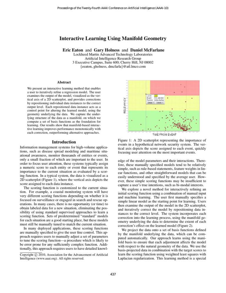
Figure 1: A 2D scatterplot representing the importance of
events in a hypothetical network security system. The vertical axis depicts the score assigned to each event, quickly
focusing user attention on the most important events.
Introduction
Information management systems for high-volume applications, such as disease spread modeling and maritime situational awareness, monitor thousands of entities or events,
only a small fraction of which are important to the user. In
order to focus user attention, these systems typically assign
a numeric score to each entity or event that represents its
importance to the current situation as evaluated by a scoring function. In a typical system, the data is visualized as a
2D scatterplot (Figure 1), where the vertical axis depicts the
score assigned to each data instance.
The scoring function is customized to the current situation. For example, a coastal monitoring system will have
very different scoring functions depending on whether it is
focused on surveillance or engaged in search and rescue operations. In many cases, there is no opportunity (or time) to
obtain labeled data for a new situation, eliminating the possibility of using standard supervised approaches to learn a
scoring function. Sets of predetermined “standard” models
for each situation are a good starting place, but these models
must still be manually tuned to match the current situation.
In many deployed applications, these scoring functions
are manually specified to give the user fine control. This approach requires users to manually adjust a set of parameters
to tune the scoring function—a procedure which is likely to
be error prone for any sufficiently complex function. Additionally, this approach requires users to have detailed knowl-
edge of the model parameters and their interactions. Therefore, these manually specified models tend to be relatively
simple, such as rule-based statements, feature weights in linear functions, and other straightforward models that can be
easily understood and specified by the average user. However, these simple scoring functions may be insufficient to
capture a user’s true intentions, such as bi-modal interests.
We explore a novel method for interactively refining an
initial scoring function using a combination of manual input
and machine learning. The user first manually specifies a
simple linear model as the starting point for learning. Users
then examine the output of the model in the 2D scatterplot,
and iteratively correct the model by repositioning data instances to the correct level. The system incorporates each
correction into the learning process, using the manifold geometry underlying the data to determine the extent of each
correction’s effect on the learned model (Figure 2).
We project the data onto a set of basis functions defined
by the manifold underlying the data, which can be computed automatically. Our approach learns using the manifold basis to ensure that each adjustment affects the model
with respect to the natural geometry of the data. We use the
basis-projected data in combination with the target scores to
learn the scoring function using weighted least squares with
Laplacian regularization. This learning method is a special
c 2010, Association for the Advancement of Artificial
Copyright Intelligence (www.aaai.org). All rights reserved.
437
(a) User scatterplot view
axis to correct its value (Figure 2). The adjusted value is
then used to refine the learned function f . The ability to
adjust the assigned score graphically allows the user to correct the current function f , as well as dynamically alter their
intended target function F in response to new or changing
information.
In visualizations where the horizontal axis embedding
represents the similarity between the data instances, the system could also enable the user to adjust the position of instances along the horizontal axis, thereby allowing the user
to correct both the value assigned to an instance as well as
its similarity to other instances. In this paper, we assume
that the user cannot graphically influence the similarity metric for the data, which is fixed after the time of manifold
construction.
(b) Underlying manifold model
Figure 2: Interactive learning of a model, showing the user
dragging two points (large light red and dark blue arrows)
and the effect on the other data points and underlying scoring function. The red adjustment has a large effect due to
the (geometrical) importance of this point, while the blue
adjustment affects only points on the local peak.
Learning the Scoring Function
While the interaction mechanisms provide a means for the
user to correct the value assigned to a single instance, it
would be cumbersome for the user to adjust the values of
all incorrect instances. Ideally, we want the user to correct
the value for as few instances as possible, with the system
attributing these adjustments onto the geometry underlying
the data in order to learn the scoring function f .
To enable the generalization of each correction to nearby
instances, we organize the data onto a manifold that captures the local similarities in the data. The basis functions of
this manifold capture the geometry inherent in the data. By
learning the scoring function on the manifold rather than the
raw data, we can localize each data adjustment to affect only
the local neighborhood, rather than the entire data set.
case of Belkin et al.’s (2006) Manifold Regularization that
constrains the smoothness of the learned function. Each successive change to the function updates the scatterplot, providing users with instantaneous feedback and allowing them
to interactively refine the learned function. This interactive
learning method enables the user to rapidly refine a simple initial scoring function to one of arbitrary complexity
that captures their intentions. This approach requires that
the user have general knowledge of the application domain,
but it does not require knowledge of the model’s internal
structure. Results show that our interactive learning method
monotonically improves performance with each correction,
outperforming alternative approaches.
Constructing the manifold
Mechanisms for User Interaction
We construct the underlying manifold M by representing
each data instance xi ∈ X as a vertex vi ∈ V in a graph G =
(V, A). G represents a discrete sample of the continuous
manifold M underlying the data. Each vertex in the graph G
is connected to its k-nearest neighbors, according to a radial
basis function of the local Euclidean distance between the
feature vectors, to form the adjacency matrix A:

if vi and vj are
 exp −||xi −xj ||2
2σ 2
k-nearest-neighbors
Ai,j =
(1)
 0
otherwise .
Our approach is guided by the need for simplicity of interaction between the user and the data. Interactive mechanisms
for learning should be intuitive and burden the user as little
as possible while obtaining the feedback necessary to learn.
Let the data be given by X = {xi }ni=1 , where each data
instance xi ∈ Rd .
We assume that the system provides a 2D scatterplot of
the data, where one axis (the vertical axis in this paper)
depicts the value of each instance according to the scoring
function. The other axis is a projection based either on the
data (e.g., the first principal component) or determined by
the user. Users can obtain a detailed view of a data instance’s
attributes to manually assess its score.
Initially, the user provides a simple function F̃ : Rd →
[0, 1], such as a linear model, that is an approximation to the
true (hidden) scoring function F : Rd → [0, 1] intended by
the user. The goal of interactive learning is to assist the user
in correcting the simple function F̃ to match the true function F . Each instance’s score is determined by the current
scoring function f , which starts as f = F̃ and changes in
response to the user’s corrections, ideally until f = F .
The user provides corrections to the system by selecting
a data instance and sliding it up or down along the vertical
The parameter σ controls the rate at which the affinity falls
off with increasing distance. This approach could also be
adapted to use other distance metrics besides Euclidean distance, such as the geodesic distance along the manifold as
computed by ISOMAP (Tenenbaum, et al. 2000).
Learning functions on the manifold
Once G has been constructed, we construct a set of basis
functions on the graph using techniques from spectral graph
theory (Chung 1994). These basis functions capture the various components of the graph with respect to its geometry, and are a discrete approximation to the continuous basis
functions of M. Using these components, we can represent
438
arbitrary functions on the graph, or take various C-order approximations to those functions with respect to the graph.
Using the graph’s basis rather than the raw data enables each
corrected value to affect the learned model with respect to
the geometry underlying the data.
The graph’s basis vectors are given as the eigenvectors of
the graph’s Laplacian (Chung 1994). Let nP= |V | and let
n
D be the degree matrix, formed by Di,i = j=1 Ai,j . The
graph’s normalized Laplacian L is given by the symmetric
matrix
1
1
L = I − D− 2 AD− 2 ,
to focus the fit on the lower order eigenvectors (i.e., the lowfrequency components of the graph), we regularize the least
squares fit of each eigenvector by the corresponding eigenvalue. Lower order components receive little regularization
due to their small eigenvalues, while higher order components are increasingly regularized. This approach provides a
“one-shot” method of regularizing the learned function, instead of trying various C-order approximations to Q, and
constrains the smoothness of the learned function. From our
experience, this approach provides good performance (only
slightly higher error than a fitted C-order approximation of
Q) at substantially reduced computational cost, which is essential for the interactive nature of this application.
Given Q and f , the column-vector W can be fit using
regularized weighted least squares by solving the following
optimization problem:
(2)
where I is the identity matrix. Chung (1994) also defines the
combinatorial Laplacian L = D − A. While both forms of
the graph Laplacian are valid, we found that the normalized
Laplacian L yields better results, and so we focus on it for
the remainder of this paper.
Taking the eigendecomposition of L yields L = QΛQT ,
where the columns of Q = [q1 . . . qn ] are the eigenvectors corresponding to the eigenvalues given in the diagonal matrix Λ = diag(λ1 , . . . , λn ). According to spectral graph theory, the eigenvalues λ1 . . . λn of L are real
and non-negative. Without loss of generality, we sort the
eigenvectors in non-decreasing order of eigenvalue such that
0 = λ1 ≤ λ2 ≤ . . . ≤ λn , where qi is the eigenvector corresponding to λi . The lowest-order eigenvector q1 is constant
with λ1 = 0. The eigenvectors in Q form an orthonormal
basis for L that respects the graph’s geometry.
As stated previously, the graph G represents a discrete
approximation of the continuous Riemannian manifold M
with Riemannian metric ψ that underlies the data. Each
vertex represents a location on the manifold, with edges
weighted based on the distance to its local neighbors. Let
g : M → R be a smooth function on the manifold. The
Laplace-Beltrami operator ∆ is defined to be the divergence
of the gradient of M, and can act on any smooth function g
defined on M. Hodge theory (Rosenberg 1997) implies that
g has a discrete spectrum based on the eigenfunctions of the
Laplace-Beltrami operator on M.
The Laplacian L is a discrete form of the continuous
Laplace-Beltrami operator ∆ that acts on a smooth function
f : V → R defined on G:
1 X f (u) f (v)
√ −√
Lf (u) = √
,
(3)
du v:v∼u
du
dv
W = argw min
n
X
√
Ωi,i (fi − Qi,∗ w) + || Λw||2 , (4)
i=1
where Ω is an n×n diagonal matrix that specifies the weight
of each instance, enabling us to ascribe higher weight to
those points that are adjusted by the √
user (as discussed below), Qi,∗ is the ith row of Q, and Λ serves as the regularization operator in this Tikhonov regularization problem (Wahba 1990;√Tikhonov and Arsenin 1977). The regularization term || Λw||2 acts as a weighted penalty on
the function’s average second-derivative, enforcing smoothness by scaling each eigenvector’s weight by its corresponding eigenvalue λi , thereby increasing the regularization on
higher order eigenvectors (those with larger eigenvalues)
to prevent overfitting with the high-frequency components.
This technique has been previously used in the context of
knowledge transfer by Eaton et√
al. (2008).
The regularization operator Λ is derived by constraining the smoothness of f (i.e., the L2 norm of the gradient of
f ) given by: h∇ f , ∇ f i = hf , Lf i = (Qw)T (LQw)
=
√
wT QT (QΛQT Qw) = wT IΛIw = wT Λw = || Λw||2 .
Therefore, this learning approach is equivalent to a special
case of Belkin et al.’s (2006) Manifold Regularization where
the regularization depends only on the smoothness of the
learned function f , without a penalty on the magnitude of
the solution.
Solving Equation 4 yields the optimal n × 1 weight vector
−1 T
W = QT ΩQ + Λ
Q Ωf .
(5)
where v ∼ u denotes that v is adjacent to u in G, and du
denotes the degree of u. Like the continuous g, f can also
be characterized by L’s eigenfunctions. Therefore, Q forms
a complete orthonormal basis that can be used to define f .
Using the eigenvector basis, we can write the function
f : V → R as f = QW, where f is an n × 1 vector specifying the current value for each vertex, and W is some n × 1
vector of weights over the eigenvectors. The vector f specifies the score for each vertex, with corrected instances having the user-specified value, and the scores of the remaining
instances assigned by the initial scoring function F̃ .
We fit W using weighted least squares on the eigenvector
basis Q and the values assigned to each instance. In order
The learned function f˜ : V → R is then given by f̃ = QW,
assigning a value f˜i to each instance xi . The function f˜ then
becomes f for the next round of correction by the user.
Weighting the corrected instances
In order to focus learning on the instances corrected by the
user, we ascribe higher weight to the corrected instances in
the least squares fit. The weight of each instance vi is given
by Ωi,i , forming the n × n diagonal matrix Ω used in Equations 4 and 5. We set the weights of all unadjusted instances
to be equal to 1, and weight all adjusted instances with a
scalar ω ∈ [1, ∞). The GUI allows the user to vary ω on a
439
where v̂j represents instance x̂j
of q̂i , and

 exp −||x−x̂j ||2
2
2σ
wj =
 0
log scale via a slider bar, enabling the user to interactively
explore the amount of generalization for the adjustments and
dynamically view the resulting model as ω varies. Our experiments show that learning using the manifold basis yields
stable results as ω varies from 10 to 10, 000 (three orders of
magnitude), rendering it unnecessary to precisely fit ω.
∈ X̂, q̂i (v̂j ) is the jth value
if x̂j is a k-nearestneighbor to x
otherwise
.
The value of the scoring function for data instance x is then
Scaling to large volumes of data
Applying this approach to large volumes of data presents a
challenge for modeling the graph structure underlying the
data and maintaining interaction with the user. The size of
the adjacency matrix A for the underlying graph grows with
the square of the number of data instances. Fortunately, A
can be efficiently stored as a symmetric banded matrix, since
each data instance is connected to its k nearest neighbors,
substantially reducing the storage requirements.1 The reverse Cuthill-McKee algorithm (1969) can be used to reduce
the full A matrix to a symmetric banded form. The graph
Laplacian L is therefore also a symmetric banded matrix,
and its eigendecomposition can be accomplished efficiently
using standard sparse eigen-solvers, such as Lanczos methods. This approach was previously used by Shi and Malik (1998) for efficient image clustering.
While this approach enables the efficient construction and
storage of the manifold underlying the data, and the efficient computation of its basis vectors, it yields a full matrix Q of the eigenvectors. Learning the scoring function
using a full matrix for Q incurs a substantial cost, which
threatens the interactive nature of the learning. Using a Corder approximation of the matrix Q (keeping only the C
lower order components, corresponding to those eigenvectors with smaller eigenvalues) will reduce the computational
cost of learning via Equation 5, but sacrifices the detailed fit
afforded by the higher order eigenvectors.
The Nyström approximation (Baker 1977; Fowlkes et al.
2004) enables us to sample the data instances and learn
on a portion of the complete manifold. We can then approximate the scoring function at all other data instances.
This approach also enables us to extend f to new data instances. Let X̂ ⊆ X be a sample of the data instances
sufficient to capture M’s underlying structure. Using the
procedure described in the previous section, we can construct the graph Ĝ underlying X̂, form a set of basis functions Q̂ = [q̂1 . . . q̂|X̂| ] over Ĝ with eigenvalues Λ̂ =
fˆ(x) =
1
|X̂|
X
λ̂i |X̂|
j=1
wj q̂i (v̂j ) ,
q̂i (v)Ŵi .
(7)
i=1
The above procedure will allow the user to adjust the
value of any instance included in the sample X̂ and have
that correction affect the learning of f̂ . However, since all
instances are displayed to the user in the scatterplot, regardless of whether they are included in the sample, we must
also provide a method for users to adjust the value of instances in X c . When a user chooses to adjust an instance in
X c , we explicitly add that instance’s eigenvector representation (computed via Equation 6) into Q̂ as an additional row,
thereby allowing the adjustment to affect the learning of f̂ .
Evaluation
Our experiments show that interactive manifold-based learning rapidly corrects the learned function f as compared to
several alternative approaches. As the starting model F̃ for
learning, we fit a linear regression model to the data, using a ridge parameter of 10E-8 for regularization. Then, a
simulated user repeatedly selects the “most incorrect” data
instance that has not yet been adjusted and drags that instance to the correct value. The correct values are given by
the true target function F , which is specified by the ground
truth values in each data set. Users are adept at identifying
data that are grossly incorrect, motivating our simulation of
a user adjusting the instances in order from highest to lowest error. After each adjustment, the model f is retrained
and evaluated against the true target function F .
Table 1 describes the data sets used in the evaluation. The
attribute values of each2 data set were normalized to lie in
[0, 1]. Since each experiment uses all available data and the
learning is deterministic, there is one “most incorrect” adjustment sequence for each algorithm and data set pairing.
Our interactive learning approach uses weighted least
squares with Laplacian regularization on the manifold basis to learn f . The data manifold is constructed using k = 3
and σ = 1. We compare interactive learning using the manifold basis to interactive learning using two alternative approaches: support vector regression (SVR) with an RBF
kernel (γ = 0.01), and least squares regularized with a
ridge parameter of 10E-8 on the base feature set X (ablating the manifold basis). We used the implementation
of these algorithms with their default parameters from the
Weka toolkit (Witten and Frank 2005). For each method, we
varied the weight ω assigned to adjusted instances from 1 to
1, 000; unadjusted instances have a weight of ω = 1.
diag(λ̂1 , . . . , λ̂|X̂| ), and learn a function f̂ = Q̂Ŵ on Ĝ
(Equation 5). The Nyström method enables us to extend the
basis vectors of Ĝ and the learned function fˆ to the remaining (or new) data instances X c = X −X̂. For a data instance
x ∈ X c , represented by vertex v, the value of eigenvector
q̂i at v is given by
q̂i (v) =
|X̂|
X
(6)
1
Note that the band’s width may be larger than k since a vertex
may be connected to more than k other vertices.
2
With the exception of the Pyrimidines data set, whose attribute
values already are in [0, 1].
440
Name
CPU
Heart Disease
Pharynx
Pyrimidines
Sleep
Wisconsin Breast Cancer
#Inst
209
303
195
74
62
194
#Dim
6
13
10
27
7
32
Predicted Attr
performance
cholesterol
survival time
binding activity
danger index
survival time
Source
UCI repository (Asuncion and Newman 2007)
UCI repository (Asuncion and Newman 2007)
Kalbfleisch and Prentice (1980)3
King et al. (1992)3
StatLib archive
UCI repository (Asuncion and Newman 2007)
Table 1: Data sets
(a) CPU
(b) Heart Disease
(c) Pharynx
(d) Pyrimidines
(e) Sleep
(f) Wisconsin Breast Cancer
Figure 3: Comparison of interactive learning performance when adjusting the “most-incorrect” instance. We measured the root
mean squared error (RMSE) of the three interactive learning methods, each for four values of ω, to the true function F .
As shown in Figure 3, manifold-based interactive learning rapidly reduces the error of the learned model, while
the alternative methods are slow to improve performance.
With one exception (SVR on CPU after 10 corrections),
manifold-based learning achieves better performance than
the other methods in all cases. Most importantly, manifoldbased learning monotonically reduces the error with each
correction. The other methods induce radical jumps in performance with subsequent corrections, often decreasing the
model’s performance before improving it. From the user’s
perspective, any decrease in performance (even temporarily)
from a correction reduces trust in the learning method. For
this reason, the results on all data sets, including CPU, support the use of manifold-based interactive learning over the
other approaches. Although it is not visible in Figure 3, the
alternative methods do eventually improve performance, but
only once most instances have been corrected.
Additionally, our results show that manifold-based interactive learning is stable to perturbations of the weight ω for
the corrected instances over three orders of magnitude, from
ω = 10 to ω = 10, 000. The performance of manifoldbased learning with ω = 10, 000 was identical to its performance under ω = 1, 000 while SVR and least squares
displayed even more erratic behavior, and so we omit these
results from the graphs for clarity of presentation.
We also conducted a second set of experiments that yield
insight into each method’s ability to alter the learned model
in response to user feedback. In these experiments, instead
of correcting the most-incorrect instance, the simulated user
corrects random instances (without repetition). Figure 4
shows the results of random correction on the data sets, averaged over 100 trials.
Manifold-based interactive learning is the only method
that monotonically improves performance in response to any
correction. The other methods first overfit the corrected data,
3
Also available from the Weka data set collection at
http://www.cs.waikato.ac.nz/ml/weka/index datasets.html
441
(a) CPU
(b) Heart Disease
(c) Pharynx
(d) Pyrimidines
(e) Sleep
(f) Wisconsin Breast Cancer
Figure 4: Comparison of interactive learning when adjusting a random instances to the correct value, averaged over 100 trials.
decreasing the model’s performance, until there are enough
corrected instances to avoid overfitting. This experiment reveals the ability of manifold-based interactive learning to
temper the effect of any single adjustment, allowing it to
have a large impact only if justified by the geometry underlying the data. Additionally, in practical use, the user may not
always adjust the most-incorrect instance, as explored in the
first experiment. Most likely, an actual user will vary somewhere between these two selection methods (most-incorrect
and random), and the results in Figure 4 show that we may
expect all user corrections to improve performance under
manifold-based interactive learning.
vides a means for the user to adjust the model over time and
for the system to use each adjustment to the maximum effect. Additionally, active learning starts with unlabeled data
and no model; interactive learning starts with unlabeled data
and an incorrect model. In this manner, interactive learning
is complementary to active learning.
Interactive learning is a relatively unexplored branch of
machine learning, bridging between automated learning and
human-computer interaction. One key dimension of variability in interactive learning approaches is the amount of
modeling expertise they require of the user. On one end of
the spectrum, users treat the modeling process as a black
box and interact only with the model’s output; our interactive learning approach belongs in this category. Another example is the interactive classifier by Fails and Olsen (2003)
for object recognition in images. In their system, users repeatedly draw rough sketches of objects, and then correct
the resulting recognition boundaries based on the metaphor
of coloring with crayons. In desJardins et al.’s (2008) interactive visual clustering, users move data instances in a
spring-embedding layout to correct the model’s output. The
system infers constraints based on the user’s adjustments,
which are then used in constrained clustering to iteratively
refine the partitioning.
At the other end of the spectrum, users interact directly
with the internals of the model, enabling fine control over
the resulting model, but requiring high levels of expertise in
modeling. For example, Ware et al.’s (2001) interactive tool
Related Work
The interactive learning framework we have described bears
resemblance to active learning, with several important distinctions. Active learning (Cohn, et al. 1996; McCallum
and Nigam 1998; Tong 2001) seeks to selectively choose
instances for labeling by a “teacher” in order to increase
the model’s performance using the minimum number of labeled instances. Active learning is driven by automation—
the learning algorithm selects the instances for labeling.
In contrast, interactive learning is user-driven—the user
chooses the adjustments to the model. Interactive learning
starts with an initial model and assists the user’s exploration
of refinements. The initial model may be entirely correct at
the time of its creation, but changes in the target concept may
reduce its correctness over time; interactive learning pro-
442
for decision tree construction allows the user to control each
split in the decision tree; the system visualizes the classification boundaries of each possibility to support the user’s
choice. Interactive feature selection (Dy and Brodley 2000)
and ensemble construction (Talbot et al. 2009) provide the
user fine control over other learning steps. The CueFlik system (Fogarty et al. 2008) for image search lies in the middle
of the spectrum by allowing users to create individual filtering rules based on training data chosen by the user.
6th ACM SIGKDD International Conference on Knowledge
Discovery and Data Mining, 360–364. ACM Press.
Eaton, E.; desJardins, M.; and Lane, T. 2008. Modeling
transfer relationships between learning tasks for improved
inductive transfer. In Proc. of the 19th European Conference
on Machine Learning, 317–332. Springer-Verlag.
Fails, J. A., and Olsen, Jr., D. R. 2003. Interactive machine
learning. In Proc. of the 8th International Conference on
Intelligent User Interfaces, 39–45. ACM Press.
Fogarty, J., Tan, D. S., Kapoor, A., and Winder, S. 2008.
CueFlik: Interactive concept learning in image search In
Proc. of the 26th SIGCHI Conference on Human Factors in
Computing Systems, 29–38. ACM Press.
Fowlkes, C.; Belongie, S.; Chung, F.; and Malik, J.
2004. Spectral grouping using the Nyström method. IEEE
Transactions on Pattern Analysis and Machine Intelligence
26(2):214–225.
Kalbfleisch, J. D., and Prentice, R. L. 1980. The Statistical
Analysis of Failure Time Data. John Wiley & Sons.
King, R. D.; Muggleton, S.; Lewis, R. A.; and Sternberg,
M. J. 1992. Drug design by machine learning. Proc. of the
National Academy of Science U.S.A. 89(23):11322–11326.
McCallum, A., and Nigam, K. 1998. Employing EM in
pool-based active learning for text classification. In Proc. of
15th International Conference on Machine Learning, 359–
367. San Francisco, CA: Morgan Kaufmann.
Rosenberg, S. 1997. The Laplacian on a Riemannian Manifold. Cambridge University Press.
Shi, J., and Malik, J. 1998. Motion segmentation and tracking using normalized cuts. In Proc. of the 6th International
Conference on Computer Vision, 1154–1160. IEEE Press.
StatLib archive. http://lib.stat.cmu.edu/datasets/.
Talbot, J., Lee, B., Kapoor, A., and Tan, D. S. 2009.
EnsembleMatrix: Interactive visualization to support machine learning with multiple classifiers In Proc. of the 27th
SIGCHI Conference on Human Factors in Computing Systems, 1283–1292. ACM Press.
Tenenbaum, J. B.; de Silva, V.; and Langford, J. C. 2000.
A global geometric framework for nonlinear dimensionality
reduction. Science 290(5500):2319–2323.
Tikhonov, A., and Arsenin, V. 1977. Solution of Ill-posed
Problems. Winston & Sons.
Tong, S. 2001. Active Learning: Theory and Applications.
Ph.D. Dissertation, Stanford University.
Wahba, G. 1990. Spline Models for Observational Data.
Number 59 of CBMS-NSF Regional Conference Series in
Applied Mathematics. SIAM.
Ware, M.; Frank, E.; Holmes, G.; Hall, M.; and Witten, I. H.
2001. Interactive machine learning: Letting users build classifiers. International Journal of Human Computer Studies
55(3):281–292.
Witten, I. H., and Frank, E. 2005. Data Mining: Practical
Machine Learning Tools and Techniques, 2nd Edition. San
Francisco, CA: Morgan Kaufmann.
Conclusion
Using the manifold basis enables interactive learning to refine the learned model based on the geometry underlying the
data. The results show that this approach improves the performance of the learned model with each correction, unlike
alternative approaches. However, we leave a rigorous proof
that this method will improve performance with each correction to future work. Our future work will also explore
and evaluate methods for handling concept drift and switching target concepts. Additionally, we intend to explore other
approaches to incorporating user interaction into learning.
Acknowledgments
This research was supported by internal funding from Lockheed Martin and NSF ITR-0325329. This work is based on
methods developed as part of Eric Eaton’s dissertation research at the University of Maryland Baltimore County, in
collaboration with Marie desJardins and Terran Lane. We
thank Sergey Malinchik for discussions on the user interface, and the reviewers for their insightful comments.
References
Asuncion, A., and Newman, D. 2007. University of California Irvine (UCI) machine learning repository. Available
at http://www.ics.uci.edu/∼mlearn/MLRepository.html.
Baker, C. T. H. 1977. The Numerical Treatment of Integral
Equations. Oxford: Clarendon Press.
Belkin, M.; Niyogi, P.; and Sindhwani, V. 2006. Manifold
regularization: A geometric framework for learning from labeled and unlabeled examples. Journal of Artificial Intelligence Research 7:2399–2434.
Chung, F. R. K. 1994. Spectral Graph Theory. Number 92 in
CBMS Regional Conference Series in Mathematics. Providence, RI: American Mathematical Society.
Cohn, D. A.; Ghahramani, Z.; and Jordan, M. I. 1996. Active learning with statistical models. Journal of Artificial
Intelligence Research 4:129–145.
Cuthill, E., and McKee, J. 1969. Reducing the bandwidth
of sparse symmetric matrices. In Proc. of the 24th National
Conference of the ACM, 157–172. New York, NY: ACM.
desJardins, M.; MacGlashan, J.; and Ferraioli, J. 2008. Interactive visual clustering for relational data. In Constrained
Clustering: Advances in Algorithms, Theory, and Applications, 329-356. Chapman & Hall.
Dy, J. G., and Brodley, C. E. 2000. Visualization and interactive feature selection for unsupervised data. In Proc. of the
443