Proceedings of the Twenty-Fourth AAAI Conference on Artificial Intelligence (AAAI-10)
Learning Discriminative Piecewise Linear Models with Boundary Points
Kun Gai and Changshui Zhang
State Key Laboratory on Intelligent Technology and Systems
Tsinghua National Laboratory for Information Science and Technology (TNList)
Department of Automation, Tsinghua University, Beijing 100084, China
gaik02@mails.thu.edu.cn, zcs@mail.thu.edu.cn
Abstract
1974; Escobar and West 1995; Neal 1992). DPM is a nonparametric mixture model with countably infinite number of
clusters, and the actual number of clusters can be automatically determined by the Bayesian posterior inference. More
details of DP and DPM can be found in (Teh 2007).
Original DPM aims to model distributions over observed
data. In regression and classification, when observed data
contain both covariates, x, and responses, y, using DPM to
model joint distribution of x and y yields generative nonparametric method for regression (Müller, Erkanli, and West
1996) and classification (Shahbaba and Neal 2009). In the
DPM classification model proposed by Shahbaba and Neal
(2009), the whole data are divided into different clusters, and
in each cluster they use a Gaussian form and a logit linear
form to model the marginal distribution of x, P (x), and the
conditional distribution of y given x, P (y|x), respectively.
Such generative method puts much focus on modeling the
marginal distribution P (x), which is indeed not required in
prediction. Imagine an area where the relation between y
and x is linear, but the distribution of x can not be well fitted by a single Guassian form. This area will tend to be
split into several smaller clusters by the Bayesian inference.
So the final decision surface tends to be more complex than
required, and the confidence of result P (y|x) will also be influenced due to smaller number of data in each cluster. Alternatively, discriminative methods, which only model the
conditional distribution P (y|x) or the decision surface, are
usually more effective towards the goal of prediction performance. One may ask: could we construct a discriminative
model, with the feature of automatically determining model
complexity brought by DPM?
We develop a two-step method to construct a discriminative model for binary classification using the Dirichlet process mixtures. In the first step, we sample some certain
boundary points which lie between positive and negative
data, and also their normal vectors which indicate normal
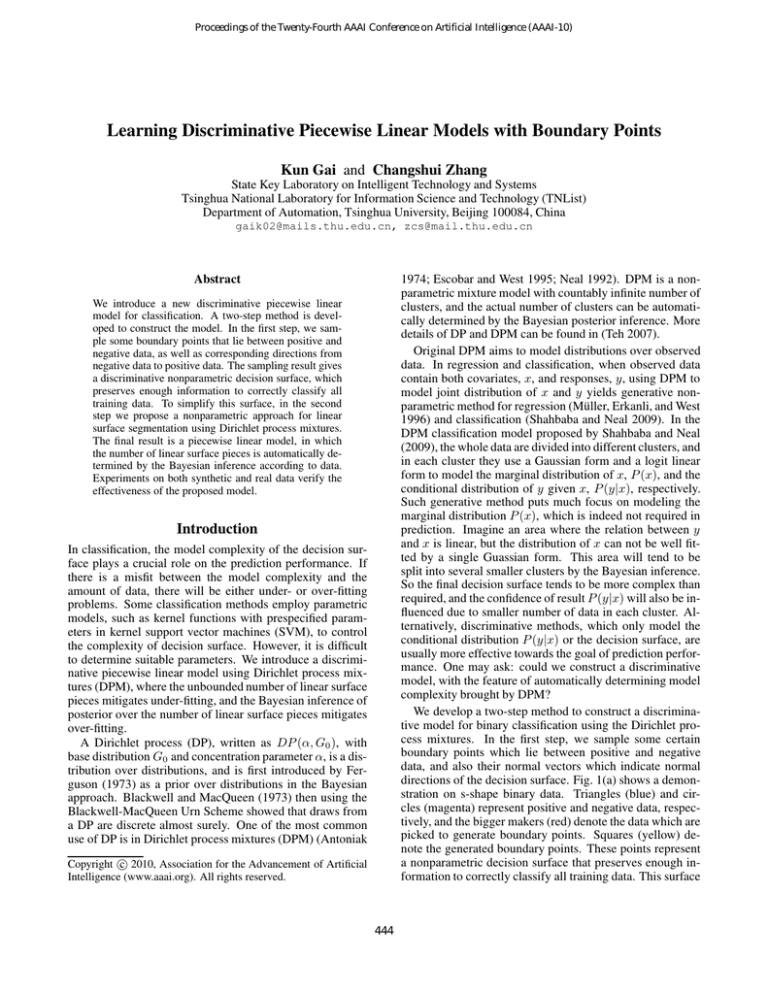
directions of the decision surface. Fig. 1(a) shows a demonstration on s-shape binary data. Triangles (blue) and circles (magenta) represent positive and negative data, respectively, and the bigger makers (red) denote the data which are
picked to generate boundary points. Squares (yellow) denote the generated boundary points. These points represent
a nonparametric decision surface that preserves enough information to correctly classify all training data. This surface
We introduce a new discriminative piecewise linear
model for classification. A two-step method is developed to construct the model. In the first step, we sample some boundary points that lie between positive and
negative data, as well as corresponding directions from
negative data to positive data. The sampling result gives
a discriminative nonparametric decision surface, which
preserves enough information to correctly classify all
training data. To simplify this surface, in the second
step we propose a nonparametric approach for linear
surface segmentation using Dirichlet process mixtures.
The final result is a piecewise linear model, in which
the number of linear surface pieces is automatically determined by the Bayesian inference according to data.
Experiments on both synthetic and real data verify the
effectiveness of the proposed model.
Introduction
In classification, the model complexity of the decision surface plays a crucial role on the prediction performance. If
there is a misfit between the model complexity and the
amount of data, there will be either under- or over-fitting
problems. Some classification methods employ parametric
models, such as kernel functions with prespecified parameters in kernel support vector machines (SVM), to control
the complexity of decision surface. However, it is difficult
to determine suitable parameters. We introduce a discriminative piecewise linear model using Dirichlet process mixtures (DPM), where the unbounded number of linear surface
pieces mitigates under-fitting, and the Bayesian inference of
posterior over the number of linear surface pieces mitigates
over-fitting.
A Dirichlet process (DP), written as DP (α, G0 ), with
base distribution G0 and concentration parameter α, is a distribution over distributions, and is first introduced by Ferguson (1973) as a prior over distributions in the Bayesian
approach. Blackwell and MacQueen (1973) then using the
Blackwell-MacQueen Urn Scheme showed that draws from
a DP are discrete almost surely. One of the most common
use of DP is in Dirichlet process mixtures (DPM) (Antoniak
c 2010, Association for the Advancement of Artificial
Copyright Intelligence (www.aaai.org). All rights reserved.
444
(a) Sampling boundary points
(b) Piecewise linearization
Figure 2: Demonstration of the support point pair (s+
i and
b
s−
),
the
edge
point
e
and
the
boundary
point
x
.
i
i
i
Figure 1: Demonstration of our two-step method.
Sampling strategy
For any input instance xi , without loss of generality, suppose xi is a positive instance, xi ∈ D+ , and consider the
following question: which instance in the training set is most
dangerous to xi , i.e., will most influence the final decision
surface towards misclassifying xi ?
To make the question tractable, we employ the simple and
powerful nearest neighbor principle. Suppose xi is removed
from the training set D, and we use nearest neighbor classifier to classify xi . The prediction of xi will be determined
−
by the relation between d+
i and di , which is defined as:
.
d+
minxj ∈D+ ,j6=i kxj − xi k,
(1)
i =
.
d−
(2)
i = minxj ∈D − kxj − xi k.
is very complex, and thus we want to combine boundary
points in local areas together to yield a local linear surface
with more generalization ability. To achieve this, in the second step we use a new DPM model to piecewise linearize
the point set surface, and finally get a piecewise linear model
for classification, as shown in Fig. 1(b) (where colors denote
different components in the mixture model).
The proposed method brings several interesting points to
related problems. First, usually only a small number of
training data are selected to generate boundary points, and
these selected data preserve zero error on all training data
and a bounded generalization error when Nearest Neighbor (NN) principle is used, which results in a new pruning
strategy for NN classifier. Second, the piecewise linearization approach using DPM provides a new nonparametric
model for subspace segmentation, which is “a fundamental problem in many applications in computer vision (e.g.,
image/motion/video segmentation), image processing (e.g.,
image compression), and systems (e.g., hybrid system identification)” (Vidal, Ma, and Sastry 2005). Finally, the introducing of boundary points gives a link between generative
and discriminative models: a generative model for boundary
points results in a discriminative model for classification.
The rest of this paper is organized as follows. First, a
novel strategy of sampling boundary points is presented.
Second, we propose a nonparametric Bayesian approach for
piecewise linearization using DPM. Then, the performance
of the proposed model on real data sets is shown. Finally,
we close with a conclusion.
+
If d−
i is smaller than di , xi will be misclassified to negative
instance. So the most dangerous instance to xi is the negative instance which determines the value of d− , i.e., is the
nearest instance with a different label. Such most dangerous
instance is called xi ’s negative support point, denoted by s−
i
(see Fig. 2 for example), and it satisfies
s−
i = arg minxj ∈D − kxj − xi k.
(3)
The instance xi and its negative support point s−
i are predicted by NN classifier (with the whole training set) to be
positive and negative, respectively. So the line segment from
xi to s−
i must cross the decision surface of nearest neighbor
principle. Then we want to obtain the intersection point.
There are some properties that are helpful to find it.
Property 1 For any point z that lies on the line segment
between a positive instance xi and its negative support point
−
s−
i , the nearest negative training instance of z is si , i.e., for
−
any z = λxi + (1 − λ)si (0 ≤ λ ≤ 1), it satisfies
Sampling boundary points
kz − s−
i k = minxj ∈D − kz − xj k.
Consider a training set D = {(x1 , y1 ), (x2 , y2 ), · · · ,
(xn , yn )}, where xi is an instance of the d-dimension input space Rd and yi ∈ {+, −} is its corresponding class
label. For convenience, the training set is divided into a pos.
itive set D+ = {xi |yi = +, (xi , yi ) ∈ D} and a negative set
− .
D = {xi |yi = −, (xi , yi ) ∈ D}, and D = D+ ∪D− . With
these training sets, we present a strategy to sample boundary
points that lie between positive and negative instances. Then
we will prove that the sampling result preserves enough information to correctly classify all training data and to classify new test data with a bounded error rate.
(4)
According to Property 1, the predicting label of any point z
on the line segment from xi to s− is determined by whether
we can find a positive training instance xk ∈ D+ that satisfies
kz − xk k < kz − s−
(5)
i k.
The perpendicular bisector of xk and s−
i can be used to
judge the correctness of (5) (note the bisector is a (d − 1)dimension linear surface, and it is a line in the 2-dimension
case in Fig. 2). Given any positive training instance xk , the
445
perpendicular bisector of xk and s−
i will intersect the bee−
line crossing xi and si (if not parallel), on the intersection
point oik , which satisfies
koik − s−
i k=
kxk − s− k2 kxi − s−
i k
−
− ,
2hxi − si , xk − si i
(6)
where h·, ·i represents the inner product. If oik is between
xi and s−
i , for any point z on the line segment between oik
and xi , it satisfies (5), and therefore is located in the positive
area of the NN principle. Considering all positive training
instances, we have the following property.
(a) Binary data
(b) Edge points
(c) Boundary points
(d) Discriminative property
Property 2 For any positive training instance xi and its
negative support point s−
i , the line segment between xi and
s−
i intersects the decision surface of NN classifier at only
one point. The intersection point is called xi ’s edge point,
denoted by ei , and it satisfies
kei − s−
i k =
minxk ∈D+ g(xk ),
s.t. g(xk ) =
−
2
kxk −s−
i k kxi −si k
−
−
2hxi −si , xk −si i
(7)
,
Figure 3: Horse Shoe data.
g(xk ) ≥ 0.
points (15.88%), in which 99 instances are support points of
themselves.
Usually the middle point of a support point pair is very
near the corresponding edge point, as shown in Fig. 2. Thus
we use the middle points as boundary points to give a more
compact representation. Fig. 3(c) shows the boundary points
by (yellow) squares. In the image, there are 92 different
boundary points, far fewer than the edge points which have
the number of 800. Besides the boundary point, the direction vector from a negative support point to a corresponding
positive support point (s+ −s− ) shows the norm direction of
the decision surface of NN classifier, which is also helpful to
represent the decision surface. Consequently, we represent
the decision surface by the following terms:
The positive training instance which is the optimal solution of (7) is called xi ’s positive support point, denoted by
s+
i . The negative and positive support points form a support
point pair. Fig. 2 shows a positive instance xi , its support
+
point pair s−
i and si , and its edge point ei . Support points
−
+
si and si are located near the decision surface of NN, and
their perpendicular bisector determines a piece of the decision surface, which is similar to support vectors in SVM and
thus is the reason why we call them support points.
Now conclude the sampling strategy. For any positive
training instance xi , use (3) to find the negative support point
s−
i , and get the optimal solution and optimal value of (7) as
−
the positive support point s+
i and the value of kei − si k,
respectively. Then the edge point is given by
−
− −1
e i = s−
ke − s−
i + (xi − si )kxi − si k
i k.
−
xbi = (s+
i + si )/2,
(8)
−
vi = (s+
i − si ),
(9)
where the boundary point xbi indicates the location that the
decision surface should cross, and vi indicates the norm direction of the decision surface on xbi . Points xbi and directions vi result in a complex nonparametric surface. To
achieve simpler representations, we will combine nearby xbi
to yield a piecewise linear decision surface using a nonparametric Bayesian approach. Before that, there are still questions to be discussed. Although edge points lie exactly on
the decision surface of NN classifier, the boundary points,
which are usually close to edge points, are not guaranteed to
be on the NN decision surface. A natural question is whether
such points xbi together with directions vi preserves enough
information for classification. Another concerned question
is: is this sampling strategy a generative or discriminative
method?
For any negative training instance, by exchanging the labels
of training instances, we still use the same strategy to get the
corresponding support point pair and edge point. The overall
computational complexity of sampling edge points and support points from n training instances is O(n2 ), which is the
same with predicting all training instances by NN classifier.
Fig. 3 shows sampling results from a horseshoe shape
data set. The original data with binary labels are shown in
Fig. 3(a). 500 positive instances, plotted by (blue) triangles,
are uniformly sampled from an M-shape area, and 300 negative instances, plotted by (magenta) circles, are uniformly
sampled from a U-shape area. The sampled support points
and edge points are shown in Fig. 3(b), where the former are
plotted by bigger (and red) markers and the latter are plotted
by (yellow) squares. As different instances may correspond
the same support point, usually only a small number of data
are selected to be support points. Besides, usually most
of support points are also support points of themselves. In
Fig. 3(b), 127 out of 800 instances are selected to be support
Zero training error and the bound of test error
Suppose we only use the support points sampled from D,
and employ NN classifier to classify all the instances in D.
446
Piecewise linearization
For any instance xi , without loss of generality, suppose it
is positive, xi ∈ D+ . Its negative support point s−
i is its
nearest negative instance in D, also in all support points.
Thus, whether xi can be correctly classified is determined
by whether we can find a positive support point closer than
+
s−
i . Since xi and its positive support point si must be in
the same side of the bisector of the support point pair (see
−
Fig. 2), s+
i must be nearer xi than si . Consequently, xi will
be correctly predicted to be positive. Now we can get:
Piecewise linear model
Now we have a decision surface represented by xbi and vi ,
where xbi indicates a point that the surface should cross, and
vi indicates the norm direction of the surface. Then we
model the decision surface by piecewise linear model using DPM. The whole model is made up by an undetermined
number of local components (cluster). In each component,
the corresponding xbi are supposed to be on a linear surface,
with the norm direction represented by w, and thus xbi should
have a very small variance at the direction w. We use a
Gaussian form which has a large precision at the direction
w to model xbi . Besides, in each component, the directions
vi are supposed to be along w with variant lengths, and thus
they have a larger variance at the direction w and smaller
variances at other directions. We use a zero-mean Gaussian form which has a small precision at the direction w and
large precisions at other directions to model vi . Considering different components, the overall model using DPM is a
piecewise linear model. Our model has the following form:
Theorem 1 Suppose the training set D satisfies: ∀ i and j,
if xi = xj , then yi = yj . We use the support points sampled
from D and employ NN principle to predict all the instances
in D, and then we will get zero error rate.
The above property shows that our sampling strategy yields
a new pruning strategy for NN classifier that preserves zero
error on the original unpruned set. The points xbi and directions vi , which are one-to-one mapped from support point
pairs, also preserve enough information for correctly classifying all training instances. This implies that the point set
surface is complex enough to mitigates under-fitting. Then,
a Bayesian approach will be used to simplify the decision
surface to further mitigate over-fitting.
With our pruning strategy, the test error is also bounded:
xbi , vi |θi ∼
θi |G ∼
G ∼
Theorem 2 Given a training set D of size N . We use the
support points sampled from D and employ NN principle to
predict new instances. This machine’s test error satisfies:
−1
E{pN
error } ≤ E{2Nsupport (D) − Nself (D)}/N,
F (θi ),
G,
DP (G0 , α).
(11)
(12)
(13)
The component parameters θ = (µ, w, λ, r, t). In our model,
the component distribution F (θ) has the form of:
p(xbi , vi |θ) = p(xbi |θ)p(vi |θ),
(10)
xbi |θ
−1
where pN
error is the probability of test error for the machine
trained on a sample of size N − 1, Nsupport (D) is the number of support points sampled from D, and Nself (D) is the
number of instances which are support points of themselves.
(14)
T −1
∼ N (µ, (λI + ww )
),
(15)
T −1
T
vi |θ ∼ N (0, ((r + t)w wI − tww )
). (16)
Here, parameters µ and w are d-dimension vectors that represent the center and the norm direction of the linear surface in each component, respectively, and parameters λ, r, t
are scalars to control precisions at the direction w and other
directions. In each component, the precision matrix of xbi
is defined by (λI + wwT ), which has a larger precision
(wT w + λ) at the direction w and smaller precision (λ) at
directions orthogonal to w. Besides, in each component the
precision matrix of vi is defined by ((r + t)wT wI − twwT ),
which has a smaller precision (rwT w) at the direction w and
lager precision ((r + t)wT w) at directions orthogonal to w.
Using such Gaussian forms, we linearize points xbi and directions vi in each component to be a linear surface piece
with the center µ and the norm direction w. The linear surface only exists locally in the corresponding component, and
the overall linearization model is a piecewise linear surface.
The base distribution G0 of DP is defined as:
The proof is given in the appendix. This theorem shows
that with proper use of support points, we can guarantee a
bounded generalization error.
Discriminative property
Generally, the strategy of sampling xbi and vi does not explore the generative mechanism of instances in D, and thus it
is a discriminative method rather than a generative method.
Fig. 3(d) gives an example. We add five gaussian components to the horseshoe shape data: the bottom one is added
to negative instances, and the rest are added to positive instances. Using such instances with a different distribution,
the sampling results of support points are the same with ones
from the original data without added components: there are
still 127 different support points, and 92 different boundary
points (However, the weights of some support points and
boundary points increase, as more instances will result in
them.). As shown in the image, the sampling strategy does
not put much focus on modeling the overall instance distribution, and directly gives representations of the decision
surface, thus the classification as a discriminative method.
p0 (θ)
λ
w
µ|λ, w
r
t
447
= p(λ)p(w)p(µ|λ, w)p(r)p(t),
(17)
∼ Gamma(αλ0 , β0λ ),
(18)
−1
∼ N (0, (P0 )
),
(19)
T −1
∼ N (µ0 , (η0 λI + η0 ww )
∼ Gamma(αr0 , β0r ),
∼ Gamma(αt0 , β0t ).
),
(20)
(21)
(22)
Although G0 is not a conjugate prior of F (θ), the Bayesian
inference of DPM with non-conjugate priors can still be handled by Markov chain approaches (Neal 2000). In our experiments, we use the Gibbs sampling method with temporary
auxiliary parameters (Neal’s algorithm 8).
Alternatively, with component distribution F (θ), if we
specify a component number and directly use G0 as the
prior rather than a DP, then we get a parametric Bayesian
mixture model for piecewise linearization or subspace segmentation. The MAP estimates of this parametric model
can be obtained through Expectation-Maximization (EM)
iterations, where the the derivation of updating equations
is straightforward and not presented here (due to lack of
space). However, in such parametric model it is difficult to
determine the component number, which explicitly controls
the model complexity. The DP prior endows us a Bayesian
way to learn the component number from data. With such
prior, the DPM model has been shown to be very effective to find a good balance between fitting accuracy and
the model complexity according to data in extensive literature, e.g., (Müller, Erkanli, and West 1996; Teh et al. 2006;
Shahbaba and Neal 2009). Thus here we use DPM to efficiently infer a reasonable component number according to
observed data.
When prediction, we want to use a fixed piecewise linear model rather than its posterior distribution for simplicity and efficiency. So we make a point estimate from the
posterior sampling results. Here we employ maximum a
posteriori (MAP) estimates for the the number of components and component parameters. After coverage, we run
the Markov chain for an enough long length, and count the
occurring frequencies of different component numbers. The
final MAP estimate of the component number is given by the
most frequently occurring one. After determining the component number, which we suppose to be K, we judge the
posterior of component parameters by
X
q(θ) =
zij p(xbi , vi |θj )p0 (θj ),
(23)
Figure 4: Piecewise linear model on synthetic data.
Then, we use the linear machine of the l-th component to
predict xt ’s label. We can use fi (x) = wiT x − wiT µi as
the linear machine for the i-th component, and the sign of
of this linear machine can be easily determined by training
instances in the i-th component. Besides, according to training instances in each component, the corresponding linear
machine can also be given by other linear classification approaches, like linear SVM. Due to the process in (24), the
computational complexity of once prediction is linear to the
number of different boundary points xbi .
Results on synthetic data
In this subsection, we illustrate our model on synthetic data.
The first data set is the horseshoe shape data set which has
been shown in Fig. 3. We run the Markov Chain for 10000
iterations, and discard the first 1000 iterations. The iterations from 1000 to 5000 is used to determine the component
number, and the Markov chain still run to iteration 10000
to refine the MAP estimates on component parameters and
component indicators of data. The overall run time is about
6 minutes (with matlab code and 3.0 Ghz CPU). Left image
in Fig. 4 shows the final result on the horseshoe shape data.
Each color represents a different component, and in all there
are six different components and six different linear surfaces
(here the linear surface is given by fi (x) = wiT x − wiT µi ).
Note the linear surface in the top (red) component is split
into two line segments by other components. So we get a
piecewise linear model that contains seven line segments.
As illustrated, the M-shape positive instances and U-shape
negative instances are almost perfectly separated by our
piecewise linear model. The right image of Fig. 4 shows the
piecewise linear model on another data set. Data are partitioned into nine components, and positive data and negative
data are perfectly separated by nine line segments. Besides,
our model on S-shape data have been illustrated in Fig. 1.
In both Fig. 1 and 4, our approach achieves high accuracies with as few linear surface pieces as possible. In all these
demo sets, if we use fewer numbers of linear surfaces than
shown, the binary data can not be well separated. Our approach gives a low and reasonable model complexity. (For
the horseshoe shape data, the authors expect 7 clusters with
7 line segments. Surprisingly, our model separates data well
using only 6 clusters.) Along with the decision surface,
more and shorter / less and longer line segments are given
to the place where the decision surface needs to turn rapidly
/ slowly, respectively. For example in Fig. 1(b), there is a
long line segment in the topmost area because one line is
i,1≤j≤K
where zij = 1 if the component indicator ci of (xbi , vi ) is
equal to j, and zij = 0 otherwise. We use the Markov chain
state which results in maximum q(θ) in the condition of K
components as estimates of component parameters, as well
as component indicators of data. In fact, after the component
number is determined, the situation is similar to the parametric model with a determined number of components. So
component parameters can also be determined by the parametric MAP approach with EM iterations.
Predicting rule
Using MAP estimation, we get the component number K,
and component indicator ci (1 ≤ ci ≤ K) for each data
(xbi , vi ) (1 ≤ i ≤ n), as well as the component parameters
(µj , wj , λj , rj , tj ) (1 ≤ j ≤ K) for each component. These
estimates result in a piecewise linear surface, and we want to
predict labels of new instances according to this surface. For
any instance xt , we first determine its component indicator
l by its nearest boundary point’s cluster label, i.e., l = ci∗ ,
where
i∗ = arg mini kxt − xbi k.
(24)
448
Table 1: Experiments on real data sets.
Data Set
IRIS
AUSTRALIAN
DIABETES
HEART
LIVER
Figure 5: The cluster number posterior.
enough for this large area. Then in the underside area, the
overall decision surface need to turn the direction rapidly
with more turning points, and thus more and shorter line
pieces are distributed here. In the whole space, the partitioning of clusters, line pieces’ lengths, positions and directions
are all very suitable for good separation. In all, our model
achieves a good balance between experiential accuracy and
model complexity.
SVM
Acc.
SV
92.96 96.67
79.16 91.88
68.48 85.94
71.32 96.67
60.61 98.84
DPLM
Acc.
BP
98.89 20.67
79.86 62.61
71.35 71.74
74.65 69.63
61.00 72.46
Experiments on real data
We test our model on five real data sets from UCI repository (Asuncion and Newman 2007) and Statlog data sets
(Brazdil and Gama). For comparison, we also use SVM with
RBF kernels, which is one of the most widely used nonlinear classifiers. In particular, the attributes of the data sets are
all normalized based on their maximum values. The SVM
tool we used is LIBSVM (Chang and Lin 2001). The parameter γ in RBF kernels and C in SVM are determined by
grid search based on 10-fold cross validation on the training
data.
In our model, the base distribution G0 of DP is set as:
Differences from parametric model
Some other works on parametric models can also result in
piecewise linear decision surfaces, e.g., mixtures of SVMs
in (Collobert, Bengio, and Bengio 2002) and Profile SVM
in (Cheng, Tan, and Jin 2007). Both mixtures of SVMs and
Profile SVM partition training data into a determined number of clusters (using K-means or its derivative) and then
builds linear SVM for each cluster. These methods does
not exploit discriminative information in the clustering step,
and thus the partitioning is usually not fit for building linear
classification model. In our model the partitioning is very
suitable for local linear surfaces, as has been shown. An example on horseshoe shape data can be found in (Cheng, Tan,
and Jin 2007), where Profile SVM uses 11 clusters and still
can not well separate data. Our model on horseshoe shape
data uses only 6 clusters and achieves good separation. Besides, the most significant difference between these parametric models and our nonparametric model is that, they need a
prespecified cluster number, whereas in our model the cluster number can be automatically determined by the posterior
inference from data.
λ ∼ Gamma(1 + 0.05d, (1/d + 0.05)tr(Σxm )), (25)
w ∼ N (0, tr(Σxm )I/d),
(26)
µ|λ, w ∼ N (E(xm ), (0.1λI + 0.1wwT )−1 ),
r ∼ Gamma(1 + 0.5d, 10 + 5d),
t ∼ Gamma(1 + 0.5d, 0.5 + 0.25d),
(27)
(28)
(29)
and the concentration parameter α of DP is set to be 0.1. The
basic principle of this setting is to decrease the influence of
the prior on results. The accuracies are obtained based on
10-fold cross validation. To make problems more challenging, we use only 1/10 data as training sets, and the other 9/10
data as test sets. Table 1 summarizes accuracies of SVM
and our discriminative piecewise linear model (referred to
as DPLM), as well as proportions of support vectors (SV)
in SVM and proportions between different boundary points
(BP) and training data in DPLM. Note that it is not a completely fair comparison, as parameters in SVM can be tuned
but parameters in prior of DPLM are fixed. However, DPLM
outperforms SVM in all these data sets. One probable reason is that in SVM it is difficult to choose suitable kernel parameters to avoid both over- and under-fitting, whether cross
validation is used. In DPLM, reasonable model complexity
is automatically determined by the Bayesian inference according to data, and thus our model provides better results.
Moreover, the boundary points used in DPLM are always far
less than support vectors in SVM, which makes prediction of
DPLM much faster.
Generally, the concentration parameter α of DP influences the cluster number prior. The average prior cluster
number is directly proportional to α (Teh 2007). One may
ask: what is the difference between specifying α in our
model and specifying the cluster number in parametric models?
Although α influences the cluster number prior, the cluster number posterior is expected to be mainly determined
by data in our Bayesian model. Fig. 5 shows the posterior
occurring frequencies of cluster numbers on the horseshoe
shape data when α is set to be different values. When α = 1,
the average posterior cluster number is 6.03, and the MAP
estimate is 6. Then we increase α to 10. The average posterior cluster number increases to 6.15, and the MAP estimate
is still 6. As shown, the MAP result of our model is invariant
to α to some extend, and it is mainly determined by data.
Conclusion
We develop a two-step method to construct a discriminative piecewise linear model using boundary points, where
the model complexity is automatically determined by data.
We use the unbounded number of linear surface pieces to
mitigate under-fitting, and employ the Bayesian inference of
449
posterior over the linear surface piece number to mitigate
over-fitting. Both synthetic and real data verify the effectiveness of our model.
instances that will be correctly classified in the leave-one-out
procedure. Then, applying Luntz and Brailovsky’s theorem
(Luntz and Brailovsky 1969) gives the result of Theorem 2.
Q.E.D.
Acknowledgments
References
The work was supported by the National Natural Science
Foundation of China (NSFC, Grant No. 60835002 and No.
60721003).
Antoniak, C. 1974. Mixture of dirichlet process with applications to bayesian nonparamteric problems. Annals of
Statistics 2(6):1152–1174.
Asuncion, A., and Newman, D. 2007. UCI machine learning
repository.
Blackwell, D., and MacQueen, J. B. 1973. Ferguson distributions via pólya urn schemes. Annals of Statistics 1:353–
355.
Brazdil, P., and Gama, J.
Statlog datasets.
http://www.liacc.up.pt/ML/old/statlog/datasets.html.
Chang, C.-C., and Lin, C.-J. 2001. LIBSVM: a library for support vector machines. Software available at
http://www.csie.ntu.edu.tw/ cjlin/libsvm.
Cheng, H.; Tan, P. N.; and Jin, R. 2007. Localized support
vector machine and its efficient algorithm. In Proceedings
of the 7th SIAM International Conference on Data Mining
(SDM 2007), 461–466. Philadelphia, Penn.: Society for Industrial and Applied Mathematics Publications.
Collobert, R.; Bengio, S.; and Bengio, Y. 2002. A parallel mixture of SVMs for very large scale problems. Neural
computation 14(5):1105–1114.
Escobar, M. D., and West, M. 1995. Bayesian density estimation and inference using mixtures. Journal of the American Statistical Association 90:577–588.
Ferguson, T. S. 1973. A bayesian analysis of some nonparametric problems. Annals of Statistics 1(2):209–230.
Luntz, A., and Brailovsky, V. 1969. On estimation of characters obtained in statistical procedure of recognition. Technicheskaya Kibernetica 3(6).
Müller, P.; Erkanli, A.; and West, M. 1996. Bayesian curve
fitting using multivariate mormal mixtures. Biometrika
83(1):67–79.
Neal, R. M. 1992. Bayesian mixture modeling. In the Workshop on Maximum Entropy and Bayesian Methods of Statistical Analysis, volume 11, 197–211.
Neal, R. M. 2000. Markov chain sampling methods for
dirichlet process mixture models. Journal of Computational
and Graphical Statistics 9:249–265.
Shahbaba, B., and Neal, R. 2009. Nonlinear models using
dirichlet process mixtures. Journal of Machine Learning
Research 10:1829–1850.
Teh, Y.; Jordan, M.; Beal, M.; and Blei, D. 2006. Hierarchical dirichlet processes. Journal of the American Statistical
Association 101(476):1566–1581.
Teh, Y. W. 2007. Dirichlet processes. Encyclopedia of
Machine Learning. Forthcoming.
Vidal, R.; Ma, Y.; and Sastry, S. 2005. Generalized principal
component analysis (gpca). IEEE Transactions on Pattern
Analysis and Machine Intelligence 27(12):1945–1959.
Appendix
Proof of Theorem 2. The proof follows the leave-one-out
procedure as in (Vapnik and Chapelle 2000). Remove one
instance (xi , yi ) from the training set D, use the remaining instances to construct a classification rule and then test
the removed instance. In such way we test all N instances
and finally obtain an leave-one-out error rate. Luntz and
Brailovsky (Luntz and Brailovsky 1969) proved that the
leave-one-out error is an almost unbiased estimate of the
probability of test error.
Now consider the the leave-one-out error of the classification rule in Theorem 2. Without loss of generality, we
suppose the removed instance, denoted by xi , is positive,
i.e., xi ∈ D+ . If xi is not a support point, and there exist
another positive instance xj ∈ D+ (j 6= i) that xj and xi
have the same positive support point s+
i , then xi will be correctly classified in the leave-one-out procedure. It is because
xj and its support point pair remain in the training set, and
thus its positive support point s+
i will be still selected as a
positive support point after xi is removed. As s+
i is nearer
xi than any negative instance in D, xi will be correctly predicted to be positive according to NN principle.
+
+
Let us use N + , Nsupport
and Nself
to denote the number
of positive instances in D, the number of positive support
points (selected from the whole training set D) and the number of positive self-support-points (which are the positive
support points of themselves), respectively. Then suppose
+
+
the Nself
positive self-support points and other Nsupport
−
+
+
Nself positive support points correspond to N1 and N2+
positive non-support-points, respectively. For the first group
of N1+ positive non-support-points, because their positive
support points are the different positive instances that result in the same positive support points with them, all these
N1+ instances will be correctly predicted in the leave-oneout procedure. For the second group of N2+ positive non+
+
support-points, because they correspond to Nsupport
−Nself
+
+
positive support points, there exist at most Nsupport
− Nself
positive non-support-points which have one-to-one correspondences with positive support points. Other N2+ −
+
+
Nsupport
+ Nself
positive non-support-points must have
many-to-one correspondences with positive support points,
and will be correctly predicted in the leave-one-out procedure. In all, for all positive instances, there exist at least
+
+
+
+
N1+ + N2+ − Nsupport
+ Nself
= N + + Nself
− 2Nsupport
+
+
+
(due to N1 + N2 + Nsupport = N + ) instances that will
be correctly predicted. Taking both positive and negative instances into account, there are at least N +Nself −2Nsupport
450