Learning Maps of Indoor Environments Based on Human Activity
Slawomir Grzonka and Frederic Dijoux and Andreas Karwath and Wolfram Burgard
Albert-Ludwigs-University of Freiburg, Georges-Koehler-Allee 079, 79110 Freiburg
{grzonka, dijoux, karwath, burgard}@informatik.uni-freiburg.de
Abstract
We present a novel approach to build approximate maps of
structured environments utilizing human motion and activity.
Our approach uses data recorded with a data suit which is
equipped with several IMUs to detect movements of a person and door opening and closing events. In our approach we
interpret the movements as motion constraints and door handling events as landmark detections in a graph-based SLAM
framework. As we cannot distinguish between individual
doors, we employ a multi-hypothesis approach on top of the
SLAM system to deal with the high data-association uncertainty. As a result, our approach is able to accurately and
robustly recover the trajectory of the person. We additionally
take advantage of the fact that people traverse free space and
that doors separate rooms to recover the geometric structure
of the environment after the graph optimization. We evaluate
our approach in several experiments carried out with different
users and in environments of different types.
Introduction
The problem of localizing and tracking people has recently
received substantial attention in the robotics community as
knowledge about the current position of a person and his or
her activity allows a mobile robot to improve its services to
its users. For example, the robot can better anticipate future
actions of the person. Additionally, knowledge about the
environment and the location of people can greatly support
search and rescue missions in emergency situations. Consider, for example, firefighters in a building enclosed by
smoke and fire. If a map of the environment can be constructed while the firefighters are within the building, an operator or automated system can re-route the people to the
exit in case of an emergency. Alternatively, one could use
the map of the environment to more intelligently coordinate
the actions of the rescue workers to more effectively search
the environment for potential victims and at the same time
reduce the time the rescue workers are exposed to potential
threats.
In this paper, we consider the problem of simultaneously
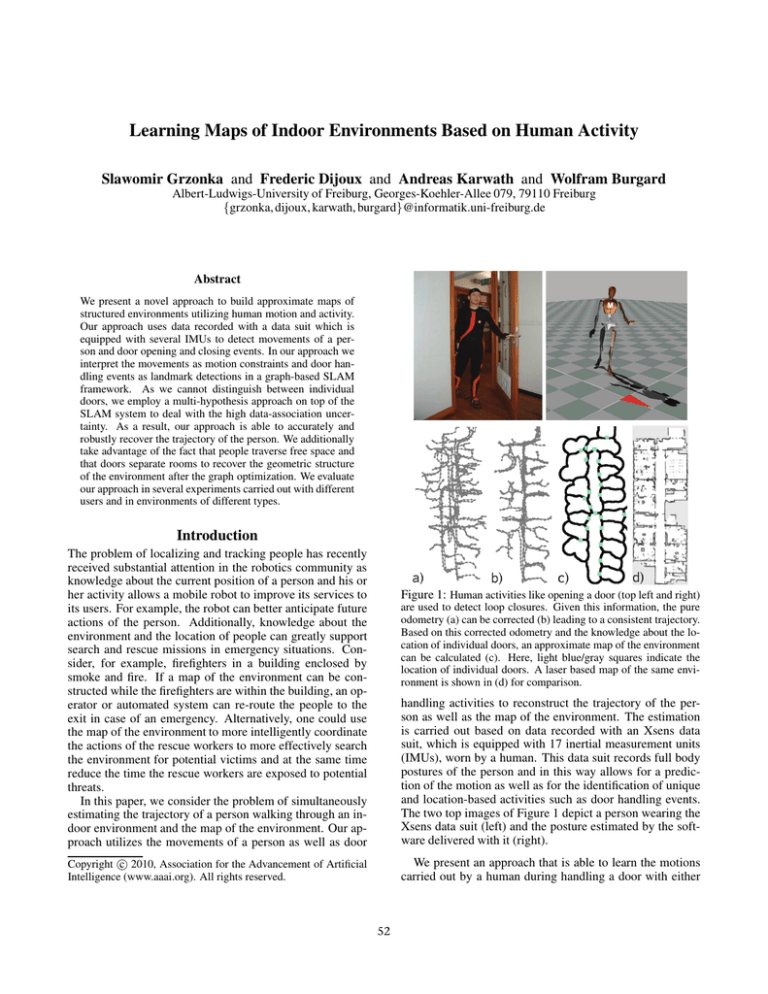
estimating the trajectory of a person walking through an indoor environment and the map of the environment. Our approach utilizes the movements of a person as well as door
Figure 1: Human activities like opening a door (top left and right)
are used to detect loop closures. Given this information, the pure
odometry (a) can be corrected (b) leading to a consistent trajectory.
Based on this corrected odometry and the knowledge about the location of individual doors, an approximate map of the environment
can be calculated (c). Here, light blue/gray squares indicate the
location of individual doors. A laser based map of the same environment is shown in (d) for comparison.
handling activities to reconstruct the trajectory of the person as well as the map of the environment. The estimation
is carried out based on data recorded with an Xsens data
suit, which is equipped with 17 inertial measurement units
(IMUs), worn by a human. This data suit records full body
postures of the person and in this way allows for a prediction of the motion as well as for the identification of unique
and location-based activities such as door handling events.
The two top images of Figure 1 depict a person wearing the
Xsens data suit (left) and the posture estimated by the software delivered with it (right).
c 2010, Association for the Advancement of Artificial
Copyright Intelligence (www.aaai.org). All rights reserved.
We present an approach that is able to learn the motions
carried out by a human during handling a door with either
52
the left or the right hand. This learned motion is then used to
detect door handling events and at the same time to estimate
the location of doors while the human is walking through the
environment. We then apply a graph-based SLAM approach
that uses the odometry estimated by the IMUs and the landmarks corresponding to the door handling events to estimate
the true path of the person. To deal with the corresponding
data association uncertainty in the landmark determination,
we apply a multi-hypothesis scheme. After calculating the
path of the person, we utilize the pose of the estimated doors
to calculate an approximate two-dimensional map of the environment.
The paper is structured as follows. After discussing related work we briefly describe the algorithms used for learning and detecting the motion for handling a door. We then review the multi-hypothesis tracker for sensors providing only
positive feedback, especially the expressions to calculate the
hypothesis probabilities. After that, we describe how we detect potential loop closure candidates and our overall system. Finally, we present our experimental results based on
real data recorded by different people walking inside and
outside of various buildings.
Figure 2: A synthetic example: Given two examples (a) and
(b) of the same motion walking. The features fl , fr are 1
(white) iff the left/right foot is in front of the body and 0
otherwise. The resulting merged template is depicted in (c).
Here, gray areas indicate the value 0.5, meaning don’t care.
Intuitively, the matrix can be interpreted through the following sections: feet parallel, right foot in front, feet parallel,
left foot in front, feet parallel.
Related Work
Motion Templates
The problem of human indoor navigation and localization
has recently become an active research field (Lee and Mase
2002; Schindler, Metzger, and Starner 2006; Liu et al. 2007;
Cinaz and Kenn 2008). A number of different sensors are
employed as well as different kind of localization techniques were used. One of the first works in this area is
the one by Lee and Mase (Lee and Mase 2002), where
wearable accelerometers and other sensors, like a digital
compass and a velocity sensor, were employed to recognize when humans perform specific activities and switch
between indoor locations. They integrate the accelerometer data over time to localize humans within a known environment, using higher level descriptors like standing 2 steps north - 40 steps east - etc. The field of indoor
navigation and localization is therefore closely related to
activity recognition using accelerometer data. (Bao 2004;
Ravi et al. 2005) present approaches to predict certain low
level activities like walking , standing, running, sit-ups, and
others using purely extracted features from raw accelerometer data and a variety of different learning algorithms. However, they do not employ this information for indoor positioning. In (Schindler, Metzger, and Starner 2006), the
authors utilize an accelerometer together with an infrared
proximity sensor mounted on a pair of headphones to detect
when a human is passing through a doorway. In this work,
the authors are able to construct topological maps, where
rooms are represented by single nodes and edges represent
the path in steps between doorways. For building these maps
and for detecting loop closures, the human user has to indicate by gesture which door was passed, i.e. giving each door
a unique identifier via the infrared proximity sensor. Within
this map, the approach also allows for localization based on
Bayesian filtering. HeadSLAM by Cinaz and Kenn (Cinaz
and Kenn 2008) employs a laser scanner together with an
IMU mounted on a helmet. They use the IMU sensor to
Since beside the current pose of the body segments no further information is available, we need to track those motions in order to detect activities like opening/closing a door.
Without this additional information we can not detect loop
closures and we can only generate an approximate map
based on the current odometry. This, however, would lead
to an inconsistent map due to small errors accumulating over
time, as shown in Figure 1(a). We therefore propose to detect the motion used for handling a door based on motion
templates (MT) as proposed by Müller et al. (Müller and
Röder 2006). The key idea of the work by Müller et al. is
to use simple boolean features like right hand is above head
and create more expressive features (motion templates) by
conjunction of the simple ones. Given f of those features
and a motion sequence of length K this leads to a matrix of
size f × K. Note that each entry of this matrix is either 1
or 0 indicating this feature being active or not at the specific
time and that the sequence length K can in general be different for each motion sequence. Consider for example the two
features fl , fr with fl indicating the left foot being in front
of the body and fr active if the right foot is in front of the
body. Given this set of features, a typical walking template
for two different sequences of the same length could look
like Figure 2(a) and (b). The learned template given these
two examples is depicted in Figure 2(c). Here, black and
white correspond to 0 and 1 respectively. The gray-shaded
boxes account for the fact 0.5 meaning don’t care. More formally, let C denote a motion class consisting of s templates
MT1 . . . MTs indicating the same motion. Each template
MTj is described by a matrix of size f × Kj and a weight
vector αj with αj (k) being the weight of the k-th column.
Initially, we set all weights to 1 indicating each time step to
be equally important. The learning of a class reference template CT is done performing the following steps. First, we
select a template MTi from the class C and use it as a refer-
be able to project the laser scans into a horizontal plane in
a global coordinate system and employ a modified GMapping (Grisetti, Stachniss, and Burgard 2005) implementation, by incorporating a simple motion model with either a
fixed speed assumption for walking or no speed while standing.
53
ence R. We then compute an optimal alignment of this reference template to all other templates from the same class utilizing Dynamic Time Warping (DTW) (Rabiner and Juang
1993). We alter the current motion template MTj (which
was aligned to R) in the following way. Given n columns of
the reference template R, namely R(k), . . . , R(k + n − 1),
are matched to one column of the current template MTj (l),
this column MTj (l) is duplicated n times having the new
weight α(l)/n. In case one column R(k) is matched to
m columns of MTj , namely MTj (l), . . . , MTj (l + m − 1),
these m columns are averaged (multiplied by their weights)
to one with the new weight being the sum of these columns’
weights. This process is called warping. Now, that each
MTj has the same length as the reference R, we calculate in
the second step a weighted average template from all templates based on the columns and their associated weights.
Consequently, this step is called averaging. In the third step,
called unwarping we stretch and contract the resulting template so that all but eventually the last column have a weight
of 1. In this case, given the weight of a column α(k) < 1,
we merge this column with subsequent ones until the weight
is 1. In case the weight of a column α(k) > 1, we duplicate
this column into two columns, one with weight 1 and the
second with weight α(k) − 1. The process is then repeated
for the next column.
We repeat the whole procedure of warping, averaging, and
unwarping for all templates MTi where every template once
is the reference template R. After this step, we replace all
templates by the outcome of the procedure when this template was the reference R. Since the selection of the reference R induces a bias on the learned template, we iterate the
whole procedure until no major change between the different templates exists. The outcome of this algorithm is the
class template CT. Note that due to the steps warping, averaging and unwarping the values of the resulting matrix are
now ∈ [0, 1] instead of ∈ {0, 1}. The final step therefore
consists of changing each entry of CT into either 0, 1 or 0.5,
with 0.5 indicating the flag don’t care. We achieve this by
selecting a threshold γ and changing each entry to 0, given
its current value < γ. The value is altered to 1 if it was
> (1 − γ) and set to 0.5 otherwise. In all our experiments
we set γ to 0.1. An example of such a template is depicted
in Figure 2(c).
Now, given the learned class template CT and a new motion sequence, we can calculate a similarity between both.
Therefore, we align the motion template of the actual sequence to CT via DTW. We obtain a score between both
templates by dividing the amount of mismatches by the
number of used cells (i.e., the cells being either 0 or 1).
Given this score is below a threshold τ , the actual motion
sequence is said to belong to the motion class CT.
Since we are only interested in the motion used for handling a door with either the left or the right hand we use
features based on the pose and velocity of the hands only.
Intuitively, we use a set of features describing whether the
hand is at the level of the door handle, whether it is raising, hold still or lowered, and finally whether the hand is
moving towards the body or away from it. We learned the
template for the activity handling a door, which consists of
the four subclasses open left, close left, open right, close
right, using 10 examples from a training data set for each
subclass. Based on a second validation data set, we selected
the threshold τ = 0.25 for detecting the motion. Using this
threshold, we did not encounter false positives on the validation data set. Although the features used for detecting a door
are quite simple, we can reliably detect the timestamp when
the door handle was touched within 1.5 seconds of the true
timestamp (i.e., manually labeled ground truth). Therefore,
we can now use the pose of the hand as an approximation
of the location of the door. Given this algorithm we are able
to detect when we touched a door, but not which one. We
therefore have to take care about possible data associations,
which is described in the next section.
Multi Hypothesis Tracking
In this section we review the Multi Hypothesis Tracker
(MHT) as described by Reid (Reid 1979) for sensors providing only positive feedback. In the original paper by Reid,
this type of sensor is called a ”type 2” sensor. There, any
measurement can be either detected (assigned to an existing
track), marked as a false alarm or as a new track. Since
in our particular case the tracks are static doors, we will
call them doors in the remainder of this section, rather than
tracks. As described in Section we select a threshold for
detection in such a way, that we do not have to model false
positives. Therefore, a measurement can only be interpreted
as detected (when matched to an existing door) or as a new
door. In order to derive the probabilities of individual measurement assignments we briefly reconsider the formulation
of the Multi Hypothesis Tracker for type 2 sensors.
Let Ωkj be the j−th hypothesis at time k and Ωk−1
p(j) the parent
hypothesis from which Ωkj was derived. Let further Ψj (k)
denote an assignment, that based on the parent hypothesis
k
Ωk−1
p(j) and the current measurement zk gives rise to Ωj . The
assignment set Ψj (k) associates the current measurement either to an existing door or a new door. Given the probability
of an assignment and the probability of the parent hypothesis Ωk−1
p(k) , we can calculate the probability of each child that
has been created through Ψj (k). This calculation is done
recursively (Reid 1979):
p(Ωkj |zk )
=
Bayes+
=
Markov
p(Ψj (k), Ωk−1
p(j) |zk )
k−1
η p(zk |Ψj (k), Ωk−1
p(j) )p(Ψj (k)|Ωp(j) ) ·
p(Ωk−1
p(j) ).
(1)
The rightmost term on the right-hand side is the recursive
term, i.e., the probability of its parent. Factor η is a normalizer. The leftmost term on the right-hand side after the
normalizer η is the measurement likelihood. We assume that
a measurement zk associated with a door j has a Gaussian
pdf centered around the measurement prediction ẑkj with innovation covariance matrix Skj , N (zk ) := N (zk ; ẑkj , Skj ).
Here, the innovation covariance matrix is the uncertainty of
the door w.r.t. the current trajectory and is described in Section . We further assume the pdf of a measurement belong-
54
Figure 3: A snapshot from our experiment which is described in detail in Section . (a) The human re-enters the building
through door A0. Based on the MHT decision new door and match with A0 different hypothesis are generated (b) and (c). The
probabilities of the hypothesis are depicted in (d).
ing to a new door to be uniform in the observation volume
V with probability V −1 . Hence, we have
p(zk |Ψj (k), Ωk−1
p(j) ) =
N (zk )δ V δ−1 ,
possible door candidates (i.e., loop closures), the calculation
of the innovation covariance and the algorithms which were
utilized in order to correct the trajectory.
(2)
with δ being 1 if and only if the measurement has been associated with an existing door, 0 otherwise. The central term
on the right-hand side of Equation (1) is the probability of an
assignment set, p(Ψj (k)|Ωk−1
p(j) ), which is composed of the
following two terms: the probability of detection pdet kj and
the probability of a new door. In our case the probability of
detection is equal to choosing one of the current candidate
doors, i.e., all doors within an uncertainty ellipsoid. There−1
, with NC(x1:k , Ωk−1
fore, pdet kj := NC(x1:k , Ωk−1
p(j) )
p(j) ) being the number of door candidates, assuming the trajectory
x1:k within the world Ωk−1
p(j) . Assuming the number of new
doors following a Poisson distribution with expected number of doors λnew V in the observation Volume V we obtain
δ
p(Ψj (k)|Ωk−1
(3)
p(j) ) = pdetk · μ(1 − δ; λnew V )
Simultaneous Localization And Mapping
We address the simultaneous localization and mapping problem by its graph based formulation. A node in the graph
represents a 3DoF pose of the human pose (i.e., the center
of the hip) or the 3DoF pose of a door and an edge between
two nodes models a spatial constraint between them. These
spatial constraints arise either from incremental odometry
or by detecting a previously observed door (i.e., by opening/closing it). In our case, the edges are labeled with the
relative motion between two nodes. To compute the spatial
configuration of the nodes which best satisfy the constraints
encoded in the edges of the graph, we utilize stochastic gradient descent optimization (Grisetti et al. 2008). Performing
this optimization whenever a door has been detected allows
us to reduce the uncertainty in the current pose estimate.
Since we are only able to detect the fact that there is a
door, we have to track different possibilities of data association, namely whether the current detected door is one of the
already mapped doors, or whether the door has not been perceived before. We therefore utilize multi hypothesis tracking as described in the previous section for all possible outcomes. To detect a potential loop closure (i.e., recognize a
previously seen door), we identify all former doors which
are within the uncertainty ellipsoid of the current pose by
a Dijkstra projection of the node covariances starting from
the current position. The innovation covariance is directly
used for calculating the likelihood of the door as described in
Equation (5). All doors being within the 99.9% confidence
region of the current pose are considered as potential loop
closure candidates, and together with the possibility of the
current detected door being a new door, give raise to n + 1
different outcomes, given the number of loop closure candidates is n. For each of these association possibilities we
create a separate graph, encode the selected constraint and
optimize it. The multi hypothesis tree therefore grows exponentially in time and pruning of this tree is mandatory in order to keep computational costs reasonable. In our case, we
utilize N-scan-back pruning as proposed by Cox and Hin-
j
(λV )n exp(λV )
is the Poisson distriwhere μ(n; λV ) :=
n!
bution for n events given the average rate of events is λV .
Therefore, Equation (1) can be reformulated into
p(Ωkj |zk )
=
Bayes+
=
Markov
p(Ψj (k), Ωk−1
p(j) |zk )
k−1
η p(zk |Ψj (k), Ωk−1
p(j) )p(Ψj (k)|Ωp(j) ) ·
p(Ωk−1
p(j) )
=
η N (zk )δ V δ−1 pδdet k (λnew V )1−δ ·
j
exp(λnew V )(1 − δ)!−1 p(Ωk−1
p(j) ). (4)
Observing that (1 − δ)! is always 1 (since δ is ∈ {0, 1}) and
noting that exp(λnew V ) can be taken into the normalizer η,
we can finally rewrite Equation (4) into
δ
k−1
p(Ωkj |zk ) = η N (zk ) pdet kj · λ1−δ
new · p(Ωp(j) ). (5)
Up to now, we can reliably detect doors and calculate the
probability of a data association. In the next section we address the remaining questions during our simultaneous localization and mapping procedure, namely the detection of
55
Figure 4: The first experiment contains a trajectory of about 1.6 km. The raw odometry is depicted in (a), whereas the most
likely trajectory based on the detected doors is visualized in (b). Based on the corrected trajectory and the knowledge about
doors, a topological map of the environment can be generated. A skeleton of the environment is generated afterwards by
enlarging the free space around the trajectory up to a maximum (c). A close-up view of the internal part is also shown in (d). A
laser map of the same enviornment is depcited in (e). A close up view of the trajectory is also shown in Figure 1.
Figure 3(d)). Here, a N-scan-back of 2 would be sufficient
to keep track of the correct data association, since the MHT
would decide to keep match with A0 at time t and discard
the other branch.
The output of this approach can be used to generate an
approximate map of the environment. Assuming that doors
separate rooms, we can cut the trajectory based on the locations of individual doors. Each segment now contains all
points belonging to one room only. Given the orientation
of a door we can merge subsequent segments which are both
connected to the same door and on the same side. In order to
seek for walls, we can furthermore enlarge the trajectory until it touches a trajectory belonging to another room or up to
a threshold d, which was set to 2.5 m in all our experiments.
An outcome of this process is shown in Figure 4(c).
gorani (Cox and Hingorani 1996), which works as follows:
The N-scan-back algorithm considers an ancestor hypothesis at time k − N and looks ahead in time to all its children
at the current time k (the leaf nodes). The probabilities of
the children are summed up and propagated to the parent
node at time k − N . Given the probabilities of the possible outcomes at time k − N , the branch with the highest
probability at time k is maintained whereas all others are
discarded. Since in our case, a step in the MHT only arises
when a door has been detected, this is identical to localize
N steps ahead in time (at door level). An example of this
approach is visualized in Figure 3. This example shows a
snapshot of one experiment which is described in detail in
Section . At the specific time t, the human walked around
the builing leaving at the top exit and entered the building
through the main entry labeled A0 in 3(a). Starting from the
pose z, where the current door was detected, the uncertainty
of the pose was back-propagated utilizing Dijkstra expansion. Since we used the same uncertainty for x and y, the
resulting ellipsoid is a circle. Note that due to the backpropagation of the uncertainty the current pose is in the uncertainty region of the door A0. For better visibility, only
the doors being considered as candidates are shown with
their uncertainty regions. Therefore, only two data associations are possible in this case, namely matching the current
door with A0, which in this case is the correct association,
or marking it as a new door. Calculating the posterior probability of each association leads to p = 0.597 for the case new
door and p = 0.403 for the correct association. A maximum
likelihood approach therefore selects the wrong association.
However, as the human enters the building and opens another door, given the previous association, different possible
outcomes are possible. Figure 3(b) depicts the situation for
the case that the previous decision was new door and Figure 3(c) shows the situation for the decision match with A0.
Given this sequence of doors, the full posterior of the branch
match with A0 at time t sums up to 0.6317 while the probability for the branch for new door sum up to 0.3683 (see
Experiments
We evaluated the approach described above on different data sets utilizing the motion of two humans including walking inside and outside of various buildings.
Videos of each experiments can be found on the web
(http://www.slawomir.de/publications/mvnVideos/). They
show the incremental update of the final best hypothesis.
Our current system, though not optimized, is able to perform
an incremental update at a rate of 10Hz on a state-of-the-art
desktop computer. The first experiment contains a trajectory
of approximately 1.6 km including 133 door actions and is
depicted in Figure 4. Given the learned motion templates,
we were able to detect 125 out of the 133 doors. The pure
odometry is shown in Figure 4(a). In this experiment, the
raw odometry is already good, since we intentionally omitted walking around tables and chairs which would result
in high pose errors due to magnetic disturbances. Therefore, a variance of 0.03 m per meter and a N-scan-back of
7 were sufficient to correct the odometry. We have chosen
λnew = 0.04 since this value is approximately obtained by
dividing the number of doors by the area covered through
the doors. Note, that although λnew is dependant on the
56
Figure 5: The second experiment containing a trajectory of about 1.3 km: the raw trajectory is depicted in (a). We intentionally
walked closely around tables and chairs resulting in a high pose error due to magnetic disturbances. The corrected trajectory
using our approach is depicted in (b). The approximate map of the environment and a floor plan of the building are shown in
(c) and (d) respectively.
building the human is operating in, small changes will not
alter the final outcome. However, if operating in a hotel,
λnew should be siginifcantly higher than if operating in a
warehouse. Based on the detection and tracking of individual doors, the map was corrected as depicted in Figure 4(b).
Note that we show the maximum likelihood map of the multi
hypothesis tracking only. Given the free space traversed by
the human and the knowledge that doors separate rooms, we
can enlarge the current trajectory up to a threshold d = 2.5 m
to seek for walls, i.e., build a Voronoi diagram, based on all
poses within a room (see Figure 4(c)). The resulting map of
the inner part is depicted in Figure 4(d). For comparison we
enlarged the indoor part of this experiment and compared it
to a laser map, which is shown in Figure 4(e) and Figure 1.
The second experiment contains a trajectory of approximately 1.3 km and was obtained by walking inside a university building containing several seminar rooms. Here, we intentionally walked closely around rows of tables and chairs.
The magnetic disturbances led to a high pose error, as can
be seen in the raw odometry (see Figure 5(a)). We therefore
used a high variance of 0.2m per meter to make sure that the
variance is not over-confident. Although the initial odometry differs up to 30m for the same place, we were able to
correct it as shown in Figure 5(b). The map obtained by our
approach is visualized in Figure 5(c) and a floor plan of the
same building is depicted in (d). In this experiment we detected all 63 doors up to an accuracy of 0.5 seconds wrt. a
manually labeled ground truth.
The third experiment contains a trajectory of a person who
is about 20cm taller than the person whose motions were
used for training the templates. The parameters used to correct this trajectory were the same as for the second experiment. The outcome of this experiment is shown in Figure 6.
Here, 24 out of 27 doors were detected.
motion. Our approach considers the trajectory of the person
as motion constraints and door handling events detected using specific motion templates as landmarks within a graphbased SLAM approach. To cope with the high data association uncertainty, we employ a multi-hypothesis tracking approach. Our approach has been implemented and tested on
real data acquired by people walking inside and outside of
various buildings. The experimental results demonstrate that
our approach is able to robustly keep track of the true data
association and accurately estimate the trajectory taken by
the person. Additionally, we can create approximate maps
of the environment which accurately resemble the true layouts.
Discussion and Future Work
Whereas the results obtained with the approach described in
this paper are very promising, there are certain limitations
and aspects that warrant future research.
The first potential line of research is to extend the approach towards three-dimensional environments. In such a
context, especially the estimation of the height of the user is
problematic according to the limitations of the current sensor technology. One way to resolve this problem and to more
accurately estimate the height could be to employ additional
activities such as the climbing of stairs to estimate vertical distances. Typically, the impacts onto the IMUs coming
from the individual steps can be detected in the accelerometer data and then be utilized to improve the height estimate.
The approach can furthermore be extended towards an unsupervised approach that clusters activities and seeks to detect loop closures based on such activities. For example, the
activities like opening a water-tab might also be detectable
in the data and could then lead to additional data associations. The only requirement would be that the objects operated by the user are stationary. Typical such activities could
be cooking or sitting on a couch.
Further improvements could be obtained in 3D by incorporating background information into the optimization pro-
Conclusions
In this paper, we presented a novel approach for approximate mapping of indoor environments using sensed human
57
Figure 6: The third experiment containing the motion from a different person. The raw odometry and the corrected trajectory
based on our approach are depicted in (a) and (b) respectively. The calculated approximate map is shown in (c) and a floor plan
of the same building is depicted in (d).
cess. For example, the individual clusters of the z values
coming from the individual floors could be used to establish
additional constraints that lead to accurate z estimates and
appropriate estimates of the the individual levels of a building.
Müller, M., and Röder, T. 2006. Motion templates for automatic classification and retrieval of motion capture data. In
Proceedings of the 2006 ACM SIGGRAPH/Eurographics
symposium on Computer animation, 137–146. Eurographics Association Aire-la-Ville, Switzerland, Switzerland.
Rabiner, L., and Juang, B. 1993. Fundamentals of speech
recognition.
Ravi, N.; Dandekar, N.; Mysore, P.; and Littman, M. L.
2005. Activity recognition from accelerometer data. In In
Proceedings of the Seventeenth Conference on Innovative
Applications of Artificial Intelligence(IAAI), 1541–1546.
AAAI Press.
Reid, D. 1979. An algorithm for tracking multiple targets.
IEEE Transactions on Automatic Control 24:843–854.
Schindler, G.; Metzger, C.; and Starner, T. 2006. A wearable interface for topological mapping and localization in
indoor environments. In Hazas, M.; Krumm, J.; and Strang,
T., eds., LoCA, volume 3987 of Lecture Notes in Computer
Science, 64–73. Springer.
Acknowledgments
The authors would like to thank Gian Diego Tipaldi for the
fruitful discussions. We would also like to thank Xsens for
providing us with the additional dataset used in the third experiment. This work has been supported by the EC under
contract number FP6-IST-034120 Micro/Nano based Systems
References
Bao, L. Intille, S. S. 2004. Activity recognition from userannotated acceleration data. 1–17. Springer.
Cinaz, B., and Kenn, H. 2008. HeadSLAM - simultaneous
localization and mapping with head-mounted inertial and
laser range sensors. Wearable Computers, IEEE International Symposium 0:3–10.
Cox, I. J., and Hingorani, S. L. 1996. An efficient implementation of Reid’s multiple hypothesis tracking algorithm
and its evaluation for the purpose of visual tracking. IEEE
Transactions on Pattern Analysis and Machine Intelligence
18(2):138–150.
Grisetti, G.; Lodi Rizzini, D.; Stachniss, C.; Olson, E.; and
Burgard, W. 2008. Online constraint network optimization
for efficient maximum likelihood mapping. In Proc. of the
IEEE Int. Conf. on Robotics & Automation (ICRA).
Grisetti, G.; Stachniss, C.; and Burgard, W. 2005. Improving grid-based slam with Rao-Blackwellized particle
filters by adaptive proposals and selective resampling. In
Proc. of the IEEE Int. Conf. on Robotics & Automation
(ICRA), 2443–2448.
Lee, S.-W., and Mase, K. 2002. Activity and location
recognition using wearable sensors. IEEE Pervasive Computing 1(3):24–32.
Liu, H.; Darabi, H.; Banerjee, P.; and Liu, J. 2007. Survey of wireless indoor positioning techniques and systems.
Systems, Man and Cybernetics, Part C: Applications and
Reviews, IEEE Transactions on 37(6):1067–1080.
58