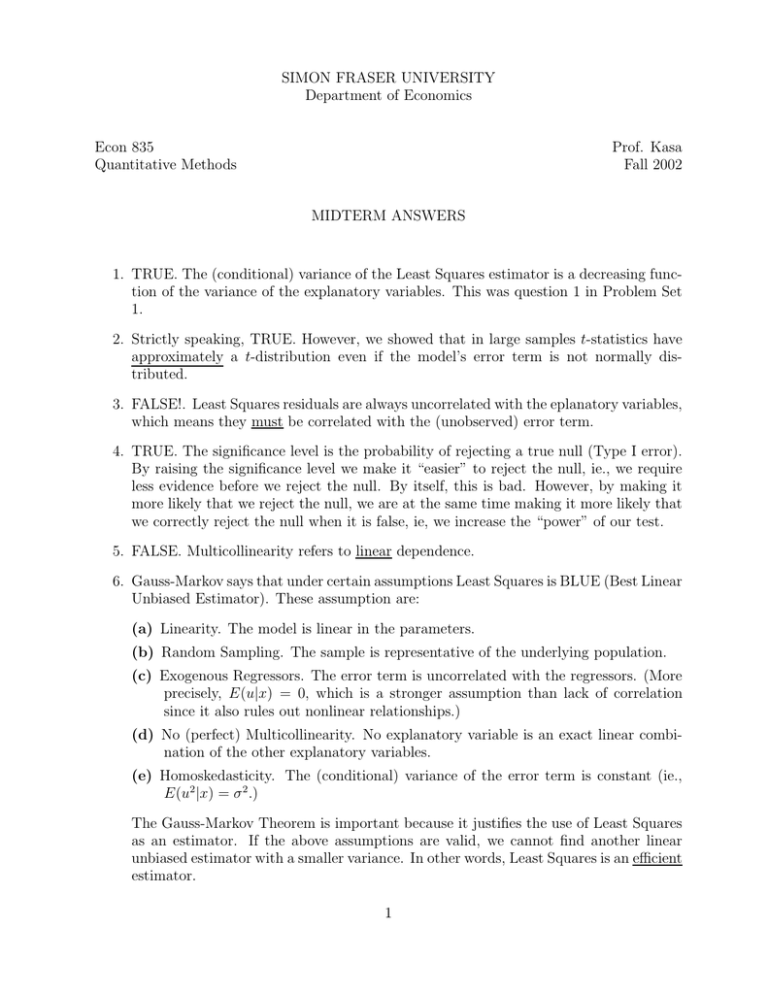
SIMON FRASER UNIVERSITY
Department of Economics
Econ 835
Quantitative Methods
Prof. Kasa
Fall 2002
MIDTERM ANSWERS
1. TRUE. The (conditional) variance of the Least Squares estimator is a decreasing function of the variance of the explanatory variables. This was question 1 in Problem Set
1.
2. Strictly speaking, TRUE. However, we showed that in large samples t-statistics have
approximately a t-distribution even if the model’s error term is not normally distributed.
3. FALSE!. Least Squares residuals are always uncorrelated with the eplanatory variables,
which means they must be correlated with the (unobserved) error term.
4. TRUE. The significance level is the probability of rejecting a true null (Type I error).
By raising the significance level we make it “easier” to reject the null, ie., we require
less evidence before we reject the null. By itself, this is bad. However, by making it
more likely that we reject the null, we are at the same time making it more likely that
we correctly reject the null when it is false, ie, we increase the “power” of our test.
5. FALSE. Multicollinearity refers to linear dependence.
6. Gauss-Markov says that under certain assumptions Least Squares is BLUE (Best Linear
Unbiased Estimator). These assumption are:
(a) Linearity. The model is linear in the parameters.
(b) Random Sampling. The sample is representative of the underlying population.
(c) Exogenous Regressors. The error term is uncorrelated with the regressors. (More
precisely, E(u|x) = 0, which is a stronger assumption than lack of correlation
since it also rules out nonlinear relationships.)
(d) No (perfect) Multicollinearity. No explanatory variable is an exact linear combination of the other explanatory variables.
(e) Homoskedasticity. The (conditional) variance of the error term is constant (ie.,
E(u2 |x) = σ 2 .)
The Gauss-Markov Theorem is important because it justifies the use of Least Squares
as an estimator. If the above assumptions are valid, we cannot find another linear
unbiased estimator with a smaller variance. In other words, Least Squares is an efficient
estimator.
1
7. This is actually a pretty deep question. You could write a dissertaion on it! It’s related
to the debate between classical (frequentist) statistics and Bayesian statistics. This is
the sort of question a Bayesian would ask. However, for this class, what I wanted you
to discuss was the idea that we want to use a procedure (ie an estimator) that performs
well on average, hoping that our particular sample is ‘typical’. The way we summarize
the average performance of an estimator is by studying its sampling distribution, ie,
the frequency distribution of estimates produced across repeated samples. Studying
the average performance of an estimator (ie contemplating its use on other samples) is
designed to avoid the potential problem of “overfitting” a particular sample.
8. If you are interested in the ceteris paribus relationship between education and wages,
then Mr Multiple is right. If experience by itself has a positive effect on wages, and
education and experience are negatively related in the sample (because it is difficult to
work and go to school at the same time), then the estimate of the returns to education
from a bivariate regression would be biased down, since on average people with more
education have less experience. Notice, however, that for some questions we may be
interested in the simple bivariate relationship. For example, if you are contemplating
going to school for another year, you may in fact want to factor in the negative impact
on earnings due to the reduced experience. In this case, the simple correlation might
be more relevant. Still, even in this case, it is useful to have the multiple regression
estimates, since they allow us to examine the effects of any hypothetical combination of
education and experience, not just the one implicitly contained in the sample bivariate
correlation.
9. Let Dm be a marriage dummy (ie Dm = 1 if the person is married and Dm = 0
otherwise. Let Dmale be a male dummy, which equals one if the person is male and
zero otherwise. For part (a) we could simply run the regression
W ages = β0 + δ · Dm + otherf actors
and test this null hypothesis H0 : δ = 0 against the alternative H1 : δ > 0.
Part (b) concerns the interaction between marriage and gender. This can be captured
by the following regression:
W ages = β0 + δ1 · Dm + δ2 · (Dm · Dmale )
where now δ1 is the marriage premium for women and δ1 + δ2 is the marriage premium
for men. Hence the null hypothesis is δ2 = 0 and the alternative is δ2 > 0.
2