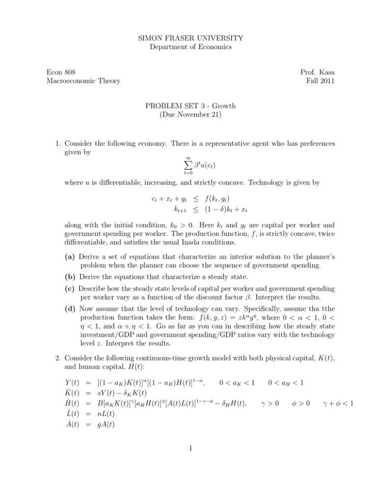
SIMON FRASER UNIVERSITY
Department of Economics
Econ 808
Macroeconomic Theory
Prof. Kasa
Fall 2011
PROBLEM SET 3 - Growth
(Due November 21)
1. Consider the following economy. There is a representative agent who has preferences
given by
∞
X
β tu(ct)
t=0
where u is differentiable, increasing, and strictly concave. Technology is given by
ct + xt + gt ≤ f (kt , gt )
kt+1 ≤ (1 − δ)kt + xt
along with the initial condition, k0 > 0. Here kt and gt are capital per worker and
government spending per worker. The production function, f , is strictly concave, twice
differentiable, and satisfies the usual Inada conditions.
(a) Derive a set of equations that characterize an interior solution to the planner’s
problem when the planner can choose the sequence of government spending.
(b) Derive the equations that characterize a steady state.
(c) Describe how the steady state levels of capital per worker and government spending
per worker vary as a function of the discount factor β. Interpret the results.
(d) Now assume that the level of technology can vary. Specifically, assume tha tthe
production function takes the form: f (k, g, z) = zk αg η , where 0 < α < 1, 0 <
η < 1, and α + η < 1. Go as far as you can in describing how the steady state
investment/GDP and government spending/GDP ratios vary with the technology
level z. Interpret the results.
2. Consider the following continuous-time growth model with both physical capital, K(t),
and human capital, H(t):
Y (t)
K̇(t)
Ḣ(t)
L̇(t)
Ȧ(t)
=
=
=
=
=
0 < aK < 1
0 < aH < 1
[(1 − aK )K(t)]α[(1 − aH )H(t)]1−α,
sY (t) − δK K(t)
γ>0
φ>0
B[aK K(t)]γ [aH H(t)]φ[A(t)L(t)]1−γ−φ − δH H(t),
nL(t)
gA(t)
1
γ+φ<1
where aK and aH are the fractions of the stocks of physical and human capital used
in the ‘education sector’, δK and δH are the depreciation rates of physical and human
capital, and B is a proportionality constant.
Notice that this model assumes that human capital is produced in its own sector with
its own production function. Raw labor (L) is useful only as something to be educated,
not as an input into the production of final goods. Similarly, knowledge (A) is useful
only as something that can be conveyed to students, not as a direct input to goods
production.
(a) Define k = K/(AL) and h = H/(AL). Derive equations for k̇ and ḣ.
(b) Derive an equation describing the set of combinations of h and k such that k̇ = 0.
Sketch it in (h, k) space. Do the same for ḣ = 0.
(c) Does this economy have a balanced growth path? If so, is it unique? Is it stable?
What are the growth rates of per capita output, physical capital, and human
capital?
(d) Suppose the economy is initially on a balanced growth path, and that there is a
permanent increase in s. How does this affect the path of per capita output over
time? Explain.
3. Consider the baseline Cass-Koopmans model,
max
c
∞
X
t=0
βt
c1−γ
t
1−γ
subject to
ct + kt+1 = zt ktα + (1 − δ)kt
(a) Derive an expression for the steady state capital/labor ratio, k̄. Use a phase
diagram to illustrate the economy’s dynamic adjustment to the steady state, with
kt on the horizontal access, and ct on the vertical access.
(b) Now let’s use DYNARE to simulate the economy’s responses to various productivity shocks. Assume that initially the economy is in a steady state with z = 1.0.
Run the program CASSKOOP1.MOD in Matlab to simulate the response to a
one-time shock at t = 0, where z0 = 1.2, and then returns back to zt = 1.0
for t ≥ 1. Assume β = 0.98, α = 0.5, and δ = 0.98. For the first simulation set
γ = 1.0, and then re-do it with γ = 5.0. Compare the two results and explain their
differences. (Hints: (1) To run dynare in matlab, just type ”dynare casskoop1” at
the matlab prompt. (2) If there is a kink at the end of simulation, try increasing
the number of periods).
(c) Now assume the productivity shock is permanent. That is, zt = 1.2 for all t ≥ 0.
This can be done by running the Dynare program CASSKOOP2.MOD. Again,
compare the results for γ = 1.0 and γ = 5.0. Which case exhibits faster convergence to the new steady state. Why? (Again: If there is a kink at the endpoint,
try increasing the number of periods).
2
(d) Finally, now assume productivity is stochastic. In particular, assume the log of
zt follows the AR(1) process zt = ρzt−1 + σεt, where ρ = 0.96 and σ = 0.01. Set
γ = 2.0, and assume all the other parameters are the same as before. Use the
Dynare program CASSKOOP3.MOD to conduct a stochastic simulation of this
model. Provide a table of auto- and cross-correlations in consumption, capital,
and productivity. Provide graphs of the impulse response functions.
4. Now let’s use dynamic programming to solve a standard growth model. Consider an
infinitely-lived representative household that owns a stock of capital, k, which it rents
to a competitive firm. Capital depreciates at rate δ. The household does not value
leisure, and supplies one unit of labor inelastically. Preferences over consumption take
the standard time-additive form, with discount factor β. The production function is
Cobb-Douglas, Yt = ztKtα Nt1−α , where zt denotes (exogenous) total factor productivity,
and Kt denotes the aggregate capital stock. (Note, in equilibrium, kt = Kt and we can
normalize N = 1).
(a) Write a Matlab program that solves the deterministic version of this model, by
setting zt = 1∀t. Set the parameters as follows: β = .95, δ = .10, u(c) =
c1−γ /(1 − γ), with γ = 3, and α = .3. Two Hints: (1) Exploit the 2nd Welfare
Theorem and compute equilibrium quantities by solving a planner’s problem, (2)
Compute the optimal policy function by first iterating on the planner’s Bellman
Equation. Make sure the capital stock grid includes the steady state, by first
solving for the steady state. Plot the the policy function, Kt+1 = g(Kt ), with
Kt+1 on the vertical axis and Kt on the horizontal axis. Also plot a 45 degree line
so as to exhibit the steady state capital stock (i.e., where Kt+1 = Kt ).
(b) Provide a sketch of the saddlepath with ∆c on the vertical axis and and ∆K
on the horizontal axis. Now compute and plot the numerical saddlepath (i.e.,
compute the function ct = h(Kt ) using the optimal policy function for Kt+1 and
the resource constraint).
(c) Re-do the above calcutions with γ = 1.01. Compare the two saddlepaths. Interpret
the results.
(d) Now suppose productivity is stochastic. Specifically, suppose z follows a 2-state
Markov chain, with zH = 1.1 and zL = 0.8. Assume the transition matrix is
P =
"
0.9 0.1
0.2 0.8
#
so, for example, P r(zt+1 = zL|zt = zH ) = 0.1. Now re-do part (a) by finding an
optimal state-contingent policy function, Kt+1 = g(Kt , zt ). Plot both g(Kt , zH )
and g(Kt , zL).
3