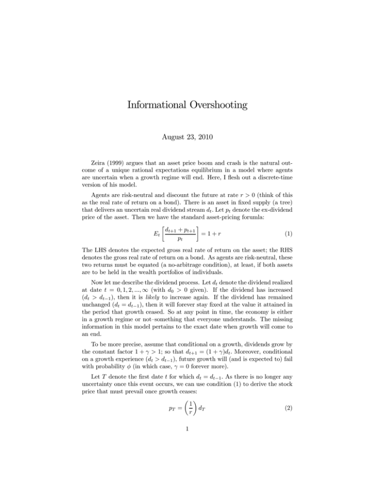
Informational Overshooting
August 23, 2010
Zeira (1999) argues that an asset price boom and crash is the natural outcome of a unique rational expectations equilibrium in a model where agents
are uncertain when a growth regime will end. Here, I flesh out a discrete-time
version of his model.
Agents are risk-neutral and discount the future at rate   0 (think of this
as the real rate of return on a bond). There is an asset in fixed supply (a tree)
that delivers an uncertain real dividend stream   Let  denote the ex-dividend
price of the asset. Then we have the standard asset-pricing forumla:
∙
¸
+1 + +1

=1+
(1)

The LHS denotes the expected gross real rate of return on the asset; the RHS
denotes the gross real rate of return on a bond. As agents are risk-neutral, these
two returns must be equated (a no-arbitrage condition), at least, if both assets
are to be held in the wealth portfolios of individuals.
Now let me describe the dividend process. Let  denote the dividend realized
at date  = 0 1 2  ∞ (with 0  0 given). If the dividend has increased
(  −1 ) then it is likely to increase again. If the dividend has remained
unchanged ( = −1 ) then it will forever stay fixed at the value it attained in
the period that growth ceased. So at any point in time, the economy is either
in a growth regime or not—something that everyone understands. The missing
information in this model pertains to the exact date when growth will come to
an end.
To be more precise, assume that conditional on a growth, dividends grow by
the constant factor 1 +   1; so that +1 = (1 + )  Moreover, conditional
on a growth experience (  −1 ) future growth will (and is expected to) fail
with probability  (in which case,  = 0 forever more).
Let  denote the first date  for which  = −1  As there is no longer any
uncertainty once this event occurs, we can use condition (1) to derive the stock
price that must prevail once growth ceases:
µ ¶
1
 =
(2)


1
for all  ≥  This is the long-run fundamental price of the asset. The question
is whether the equilibrium price may overshoot this long-run fundamental price.
If so, the price dynamics will, ex post, have resembled an asset price bubble.1
For dates    condition (1) implies
(1 − ) [(1 + ) + +1 ] +  [ +  ] = (1 + )
I conjecture an asset price function in the form of  = ( ) From the
asset-pricing equation above, this implies
(1 − ) [(1 + ) + ((1 + ))] +  [ + ] = (1 + )()
I am guessing that there is a number  (likely 1 + , but let me check) satisfying
((1 + )) = () If so, then
(1 − ) [(1 + ) + ()] +  [ + ] = (1 + )()
Now solve for () (conditional on  ),
(1 − )(1 + ) + (1 − )() +  [ + ] = (1 + )()
[1 +  − (1 − )] () = [(1 − )(1 + ) +  (1 + )] 
So,
() =
This implies that
((1 + )) =
[(1 − )(1 + ) +  (1 + )] 
[1 +  − (1 − )]

[(1 − )(1 + ) +  (1 + )] (1 + )
[1 +  − (1 − )]

Setting ((1 + )) = () and solving for  yields (as expected)  = 1 + 
And so, if the end has not been reached, the equilibrium asset price is given
by
() = Ω
where
Ω=


(3)
(1 − )(1 + ) +  (1 + )
1 +  − (1 − )(1 + )
We should check to see what happens if  = 0 (the dividend is expected to
grow forever at rate  ). In this case, our formula suggests
∙
¸
(1 + ) 
() =
−

1 (Note: when bubbles break in the data, do asset prices end up higher, lower, or at same
place as before? I would argue higher, lending support to this hypothesis over, say, a selffulfilling bubble, which places little or no restriction on where you go following a bust.)
2
which is nonsense, unless the dividend grows slower than the rate of interest. Of
course, if  = 0 then we get the standard result. In general, we have to impose
the following condition:
1 +   (1 − )(1 + )
(4)
Note that this price is proportional to the long-run fundamental price 
(assuming growth was to stop). I suspect, however, that ()   That is, the
price will be capitalizing some expected growth (even if it does not materialize,
ex post). For this to be true, the following must hold (Ω  1) :
(1 − )(1 + ) +  (1 + )
(1 − )(1 + )
(1 − )(1 + )
(1 − )(1 + )
(1 + )
1






1 +  − (1 − )(1 + )
1 +  −  (1 + ) − (1 − )(1 + )
(1 + )(1 − ) − (1 − )(1 + )
( − )(1 − )
( − ) i n d e p e n d e n t o f f a i l u r e r a t e ?
−1 t r i v i a l l y s a t i s fi e d ?
So along an equilibrium trajectory, the asset price is growing at rate   1
At any point in time, it is “over-valued” relative to a “flat” dividend profile  by
the factor Ω For the period in which growth ceases, the asset price “collapses”
by the factor Ω to its (now) long-run fundamental value.
Let me assign some numbers, let’s say, for annual data. Let  = 005
 = 006 and  = 13
Ω=
(23)(106)(005) + (13) (105)
= 112
105 − (23)106
That is, consider an asset that is growing one percent faster than the economy.
On the day grow ceases (it is now growing five percent slower than the economy),
its price drops by 12%.
How about  = 010 and 105 − (1 − )11 =   0 Set  = 0001 so that
 = 004637 In this case,
Ω=
(09537)(11)(005) + (04637) (105)
01011
=
= 100+

00010
So here, a very high rate of return with low probability of ending. The price
collapse will be huge.
3