From: AAAI Technical Report SS-03-05. Compilation copyright © 2003, AAAI (www.aaai.org). All rights reserved.
Towards a commonsense estimator for activity tracking
Catherine Tessier
Onera-Cert - BP4025 - 31055 Toulouse Cedex France
Catherine.Tessier@cert.fr
Abstract
Our purpose in this work is to track agents’ activities and to
issue a report in terms of plans or procedures that are likely to
be in progress, for applications such as surveillance, situation
assessment, hazard detection.
Starting from both Kalman filtering and Boutilier’s generalized update, a symbolic “commonsense” estimator has been
designed and implemented. The relevance of prediction is
shown for activity tracking and the symbolic estimator –
K ALMANSYMBO – is designed as a two-step (prediction and
correction) iterative process that calculates a preference relation on a set of activities, given the successive observations.
Introduction
Automatic activity tracking aims at reporting what agents
are doing thanks to observations that are perceived through
sensors or communication. Applications include surveillance, situation assessment, hazard detection, in context
such as sensitive sites, autonomous systems, pilot assistance.
For the sake of clarity, we are considering a simplified
surveillance application involving pedestrians and vehicles
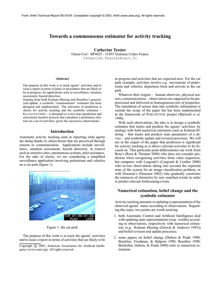
on a car park (figure 1).
in progress and activities that are expected next. For the car
park example, activities involve e.g. movements of pedestrians and vehicles, departures from and arrivals in the car
park.
Whatever their origins – human observers, physical sensors, communications – observations are supposed to be preprocessed and delivered as homogeneous sets of properties.
The translation of sensor data into symbolic information is
outside the scope of the paper but has been implemented
in the framework of P ERCEPTION project (Barrouil et al.
1998).
With such observations, the idea is to design a symbolic
estimator that tracks and predicts the agents’ activities, by
analogy with both numerical estimators such as Kalman filtering – that tracks and predicts state parameters of a device – and symbolic update and revision processes. We will
see in the sequel of the paper that prediction is significant
for activity tracking as it allows relevant activities to be focused on. This particular point differentiates our work from
Rota’s (Rota & Thonnat 2000) who does not consider prediction when recognizing activities from video sequences,
but compares with Largouët’s (Largouët & Cordier 2000)
who revises observations taking into account the expected
state of the system for an image classification problem, or
with Dousson’s (Dousson 2002) who gradually constrains
the instances of chronicles by new matched events in order
to predict relevant forthcoming events.
Numerical estimation, belief change and the
symbolic estimator
Activity tracking amounts to updating a representation of the
observed agents’ states according to observations. Regarding this topic, two points are worth noticing:
Figure 1: the car park
The purpose of this work is to track the agents’ activities
and to issue a report in terms of activities that are likely to be
Copyright c 2003, American Association for Artificial Intelligence (www.aaai.org). All rights reserved.
1. both Automatic Control and Artificial Intelligence deal
with updating state representations (resp. worlds) according to observations, respectively with numerical estimators (e.g. Kalman filtering (Grewal & Andrews 1993))
and belief revision and update processes;
2. some papers on belief change (Dubois & Prade 1998;
Boutilier, Friedman, & Halpern 1998; Boutilier 1998;
Benferhat, Dubois, & Prade 2000) refer to numerical estimation.
An extensive study of both approaches (Cossart & Tessier
1999) has shown that:
despite their different representation framework (numerical vs logic), they can indeed be compared;
update processes have tended to get closer to the principles of Kalman filtering. For instance, Boutilier’s generalized update (Boutilier 1998) and Kalman filtering:
dispersion
best state estimate
Kalman filtering:
gaussian distribution associated with state
dispersion
– are both based on an evolution model1 (a state equation, resp. a world evolution model) and an observation
model;
– both involve a two-step process – prediction and correction (resp. revision) – which consists in modifying
the uncertainty features of the representation of the
state (resp. the worlds), as time goes by and new
observations are taken into account; the best estimate
of the state (resp. the preferred worlds) is (are) the
most certain, the other ones make up the dispersion
“around” it (them) – see figure 2.
Preferred worlds
Generalized update:
preference relation associated with worlds
Figure 2: uncertainty features in Kalman filtering and generalized update
Nevertheless, some differences remain, e.g. generalized
update does not involve non-stationary models, whereas
Kalman filtering does in general; moreover, generalized update remains at a theoretical level, whereas Kalman filtering
is widely used for operational systems.
K ALMANSYMBO is inspired by both approaches: the philosophy of the Kalman filter is the basis for the prediction
and correction processes, and a preference relation on the
activities is used to represent the matching uncertainties.
K ALMANSYMBO is also inspired by commonsense: human
beings tend to predict what is likely to happen and correct
their predictions thanks to what they perceive.
Our purpose in this work is to have a more global view
on the agents’ activities, and especially on the agents’ sequences of activities. Therefore the evolution models (plans)
are sequences of activities and are equivalent to the possible “state equations” of the agents (as a reference to the
state equation in Kalman filtering), i.e represent the expected
agents’ behaviours. Activities are conjunctions of properties
which meet the “domain constraints” (Sandewall 1996) and
describe commonsense knowledge about “material objects
and their properties” (McCarthy 1989): this is quite close
to the approach described in (Santos & Shanahan 2002) for
describing the relations on physical bodies for image interpretation in a robotics context. Observations are also conjunctions of properties. Therefore a theoretical framework
to describe conjunctions of properties is needed.
Formalizing conjunctions of properties
Conjunctions of properties are well-formalized through the
cube model (Chaudron, Maille, & Boyer 2003).
Given a classical first order language (Const, Var, Funct,
Pred) with Const the set of the constants, Var the set of the
variables, Funct the set of the functions, Pred the set of
the
predicates, and Term the functional closure of Const Var
by Funct, let be the power set of the first order literals.
Definition: a logical cube2 is an element of , i.e. a
finite set of first-order positive literals.
Example: "! .
From the semantics point of view, cubes are interpreted as
the conjunction of the literals (cubes play a dual role with respect to the classical clauses). Thus, by default, the variables
are existentially quantified.
&
'
'(! is interpreted as
Example: cube $#%
')*&
',+-
'(. .
For the car park example, variables are denoted as ,
... Constants are the numbers, or denote the name
of the objects (oo1...), the type of the objects (pedestrian, vehicle...), the name of relevant places in the environment (parking-place, exit...) Predicates express elementary properties: speed(oo1,0) means that object oo1 has a
zero speed. Finally logical cubes express sets of properties:
type(oo1,vehicle) speed(oo1,x) corresponds to the logical
formula: ')213456
'78769: / 58;<=?>'58@+BA.C545$DC
78769C. , which
means that object oo1 is a vehicule and has a certain speed
.
As K ALMANSYMBO is implemented with Prolog III3 , this
syntax will be used in the paper, especially for the examples.
,/,0
Evolution models
Models and observations
Boutilier’s generalized update rests on an event-based
model: an event e maps a world w into another world w’
and is associated with a (numerical) plausibility of the occurrence of e at world w. This is a local view, as the focus is
on individual worlds and not on sequences of worlds. Moreover, the semantics of plausibilities may be hard to assess.
1
in this paper, a model is a representation of the dynamic behaviour of an agent or a system.
Definition: an activity is a logical cube. It is implemented
as act(name of plan, activity number, objects
variables, cube of properties).
Example: the second activity of plan VD (vehicledeparture) is described in Prolog as:
2
The term cube was used for the first time by A. Thayse
(Thayse & col. 1989). The term product had been used before
– but not defined – by Vere (Vere 1975).
3
c PrologIA.
act(VD, 2, <y,x>,
< type(y,pedestrian), speed(y,w),
type(x,vehicle), speed(x,v),
getting_closer_to(y,x), {v=0, w#0} >)
which means that activity VD2 holds if there is a pedestrian
with a non-zero speed moving towards a motionless vehicle.
Remark: contrary to Rota (Rota & Thonnat 2000), only
“needed variables” are considered in the activities. There
are no “forbidden variables”.
Definition: a plan is an acyclic interpreted Petri net (Murata 1989) in which places are associated to activities, and
transitions are associated to conditions representing beginnings or ends of activities.
For the car park example, we will consider a simplified
set of four plans based on very simple Petri nets (no parallelism nor choices of activities are considered), namely:
PM pedestrian-moving, VM vehicle-moving, VD vehicledeparture, VA vehicle-arrival (see last page of the paper).
Observations
Depending on the application, observations are delivered
by an observation process either asynchronously (e.g.
through communications), or synchronously (e.g. flight
data recorder), or on request (e.g. a surveillance system
supervised by human operators). The way the observations
are delivered is outside the scope of the paper, it will
be assumed that observations come at processing times
9: C .
Definition: an observation is a (partially) instantiated
logical cube. It is implemented as observation(name
of observation, processing time, cube of
properties).
Example: observation obs3 is described in Prolog as
observation(obs3, 3,
< type(oo1, pedestrian), speed(oo1,4),
type(oo2,vehicle), speed(oo2,0),
getting_closer_to(oo1,oo2) >)
which means that a pedestrian-type object oo1 with a
4km/h-speed is observed and is moving towards a motionless vehicle-type object oo2. Identifiers oo1 and oo2 are
given by the observation process.
As for Kalman filtering or generalized update, agents
(pedestrians, vehicles...) are not directly observable without error or do not behave exactly as expected. Therefore
in general, observations will not exactly match the expected
activities. K ALMANSYMBO aims at compensating for these
uncertainties and at reporting on the on-going and further activities whatever the observation may be. The main process
for that is an observation - activity matching.
Observation - activity matching
Discriminating matching conditions (i.e. conditions that
must be verified according to commonsense) are considered
so as to constrain the matching procedure to output realistic
results (depending on the application).
For the particular case of the car park, the number of agents,
their identifiers and types, and the constraints on the speed
are considered as discriminating matching conditions (i.e. a
one-agent observation will not be matched with an expected
two-agent activity, a pedestrian will not be matched with an
expected vehicle, and a motionless agent will not be matched
with an expected moving agent).
Let Obs be an observation and Act an activity. Four cases
are considered for the matching of Obs with Act:
1. Obs meets the discriminating conditions of Act and the
other properties in Obs perfectly match the other properties of Act: Obs perfectly matches Act;
2. Obs meets the discriminating conditions of Act and the set
of the other properties in Obs is either strictly included
into the set of the other properties in Act, or conversely:
Obs partially matches Act, and this kind of partial matching will be called partial(1);
3. Obs meets the discriminating conditions of Act and the set
of the other properties in Obs is neither strictly included
into the set of the other properties in Act, nor conversely:
Obs partially matches Act, and this kind of partial matching will be called partial(2);
4. Obs does not meet the discriminating conditions of Act:
matching is impossible.
Definition: the result of the matching of an observation
with a set of activities is given through a preference relation
which arranges the individual matchings, perfect matchings
being preferred to partial matchings, partial(1) matchings
being preferred to partial(2) matchings, all of them being
preferred to impossible matchings.
Notice that partial matchings and their relative preferences could be further refined depending on the application.
Example: let us consider the observation described by:
observation(obs10,10,
< type(oo22,vehicle), speed(oo22,15),
getting_closer_to(oo22, exit) >)
meaning that a vehicle-type object oo22 with a 15km/hspeed is observed and is moving towards the exit.
The matching with the activities defined in the plans (see
last page of the paper) gives the following results:
<perfect,VD,5,
< type(oo22,vehicle),
<partial(1),VM,1,
< type(oo22,vehicle),
<partial(2),VA,1,
< type(oo22,vehicle),
<partial(2),VA,2,
< type(oo22,vehicle),
speed(oo22,15) > >
speed(oo22,15) > >
speed(oo22,15) > >
speed(oo22,15) > >
The preference relation can be represented in the following classical way with the most preferred activities at the
bottom (see figure 3):
VA1 (oo22, 15)
Therefore prediction has to be considered and Kalman filtering serves as a basis to design the general principle of
K ALMANSYMBO.
VA2 (oo22,15)
K ALMANSYMBO: prediction and correction
VM1 (oo22,5)
Initialization
VD5 (oo22,15)
Figure 3: matching results - preference relation
Why matching without predicting is not
efficient
Activity tracking could be achieved with re-considering the
observation - activity matching process described above
each time a new observation comes. Nevertheless, this leads
to erratic results, as it is shown with the following example.
Example: let us consider the sequence of observations:
observation(obs21,1,
< type(oo1,pedestrian), speed(oo1,4) >)
observation(obs22,2,
< type(oo1,pedestrian), speed(oo1,0) >)
observation(obs23,3,
< type(oo1,pedestrian), speed(oo1,4),
type(oo2,vehicle), speed(oo2,0),
getting_closer_to(oo1,oo2) >)
observation(obs24,4,
< type(oo2,vehicle), speed(oo2,0) >)
observation(obs25,5,
< type(oo4,vehicle), speed(oo4,25) >)
The matching results are written in the following table,
together with comments:
Observation
obs21
obs22
Matching
perfect PM1 (oo1,4)
perfect VD1 (oo1,4)
-
Comments
OK
no result, speed
constraint not met
obs23
perfect
VD2(oo1,4)(oo2,0)
partial(2)
VD3(oo1,4)(oo2,0),
VA4(oo1,4)(oo2,0),
VA5(oo1,4)(oo2,0)
a new plan (VA) is
considered with the
same objects
obs24
perfect VD4(oo2,0)
partial(1) VA2(oo2,0),
VA3(oo2,0)
matching with VA
“has gone back in
time”
obs25
perfect DV1(oo4,25)
partial(1) VD5(oo4,25),
VA1(oo4,25),
VA2(oo4,25)
new agent, previous
ones are forgotten
The main drawback is that there is no real tracking: the
matching may give no result, or give a result that is not coherent with the plans (see what happens with VA), or definitively “forgets” previously observed agents.
Initialization of activity tracking with K ALMANSYMBO is
the plain observation - activity matching described previously. When the first observation Obs1 is considered, a
matching with all the available activities in the plans is attempted, and a first estimated situation <=1
.9 "9$ is calculated
as the preference relation # # on the matchings of Obs1.
Prediction
Let <31
be the estimated situation at processing time
: <=1
is a set of activities 6?1
arranged by the
preference relation .
from <=1
is the
The predicted situation <=1
B9
set of the predicted activities 1
9 arranged by the
preference relation # , such that:
if 6?1
is an instantiation of activity 6?1 in plan
6?1 # 6?1 6?1 , then:
a predicted activity 6?1
9 from 6?1
is
an instantiation of one of the activities of the sequence
6?1 6?1 ( '6?1 6?1 correspond to the reachable
markings from the place representing 6?1 in the Petri net
representing plan '6?1#4 6=?1 6?1 );
keeps the instantiated
the instantiation of 6?1
9
6
?
1
that correspond to properties that do
variables of
not change and releases the other ones (e.g. for the car park,
the types of the observed agents are assumed not to change
over time).
Example: predicted activities from the matched activity
<partial(2), VA,2,
< type(oo22,vehicle), speed(oo22,15)>>
are:
ACT_PREDICT(VA,2,<oo22>,
<type(oo22,vehicle), speed(oo22,X_24),
close_to(oo22, parking_space)>)
ACT_PREDICT(VA,3,<oo22>,
<type(oo22,vehicle), speed(oo22,0),
on(oo22,parking_space)>)
ACT_PREDICT(VA,4,<X_30,oo22>,
<type(X_30, pedestrian), speed(X_30,Y_30),
type(oo22,vehicle), speed(oo22,0),
close_to(X_30,oo22),
on(oo22, parking_space)>)
ACT_PREDICT(VA,5,<X_33,oo22>,
<type(X_33, pedestrian), speed(X_33,Y_33),
type(oo22,vehicle), speed(oo22,0),
moving_away_from(X\_33,oo22),
on(oo22,parking_space), {Y_33 # 0} >)
Notice that vehicle oo22 is predicted as such (no change)
and that an agent (a pedestrian) that is expected but not already observed is identified with a variable. Constraints on
the speeds are also predicted.
# extends to the predicted activities 6?1
9 , which are kept at the same relative level of preference
as activities 6?1
. Nevertheless, if the same predicted
activity with the same instantiation appears several times in
the preference relation, only the most preferred is kept.
Remark: this results in the fact that prediction tends to
“flatten” the preference relation. This compares to what
happens with the probability distribution in the prediction
step of Kalman filtering.
Depending on the dynamics of the observed agents and
on the frequency and focus of the observations, prediction
can be performed either on all the activities of the involved
plans (this is what is done for the car park example), or only
on a limited horizon (i.e. a limited number of activities in the
involved plans). The latter case is considered when temporal
data (durations, starting and ending times) are associated to
activities, as it is the case for procedures in aeronautics for
example.
Correction
Correction is the observation - activity matching when activities have been
predicted (situation <=1
9 ) and a new
observation A # comes. Four cases may arise:
1. the new observation can be matched with at least one
predicted activity (according to the matching process described previously).
In this case, the corrected situation <=1
9 9$ is the
set of the corrected activities 6?1
9 94 arranged
by the preference relation # # , such that:
activity is the result of the matching of
aA corrected
# with a predicted activity 6?1
9 ;
the preference relation # # arranges the corrected
activities from the most preferred ones (perfect matching)
to the least preferred ones ( partial(2) matching).
2. the new observation cannot be matched with the predicted
activities but can be matched with at least one other activity (according to the initialization process); this case
arises when new agents are observed (previous activities
are completed or a change of focus of the observations has
occurred).
In this case, the new situation <31
9 94 is the
set of the new activities 6?1
9 9$ arranged by the
preference relation # # , the matching and arranging
processes being the same as in the initialization process.
Nevertheless the previously predicted activities 6?1
9 are kept in order to avoid sharp changes of focus
in the estimation process in case the new activities are
not confirmed afterwards, and to allow further corrections
to be performed. At the next prediction step, the prefer # will rank the predicted activities
ence relation 1
9 at time as the most preferred ones and the
predicted activities 6?1
9$ at time 9 as the
least preferred ones .
3. the new observation cannot be matched at all, but the observed agents are already known.
In this case, <=1
9 94 is just a confirmation of
previously observed agents (types, identifiers). The pre
9 at time are kept to allow
dicted activities 6?1
further corrections to be performed. The preference relation # is the same as # .
4. the new observation cannot be matched at all and the observed agents are not known.
In this case, unexpected agents are observed; either it is
an aberrant observation, or it is something that is worth
tracking (intrusion, hazard...) For that second reason,
instead of being rejected, the observation is kept as an
activity within situation <=1
9 94 . Consequently,
if the unexpected agents are further confirmed, the
prediction and correction process will apply to their
activities. As for cases 2 and 3, the predicted activities
6?1
9 at time are kept to allow further corrections
# will
to be performed: the preference relation 6
?
1
9
first and then
rank the predicted activities
the predicted (possibly) aberrant activity.
Depending on the dynamics of the application, the predicted activities 1
9 can be kept for several time
9 6 if they are not matched with new obsersteps 2
vations. This allows the estimator to keep several tracks corresponding to agents which are not observed continuously.
Example
Only for this example, we will consider that the predicted
9 are kept for only one time step if they
activities 6?1
B
are not matched with the new observation A # .
Let us consider the following sequence of observations:
observation(obs1,1,
<type(oo1,pedestrian), speed(oo1,4)>)
observation(obs2,2,
<type(oo1,pedestrian), speed(oo1,0)>)
observation(obs3,3,
<type(oo1,pedestrian), speed(oo1,4),
type(oo2,vehicle), speed(oo2,0),
getting_closer_to(oo1,oo2)>)
observation(obs4,4,
<type(oo3,tiger), speed(oo3,5),
type(oo2,vehicle), speed(oo2,0),
close_to(oo3,oo2)>)
observation(obs5,5,
<type(oo2,vehicle), speed(oo2,0)>)
observation(obs6,6,
<type(oo4,vehicle), speed(oo4,25)>)
observation(obs7,7,
<type(oo2,vehicle), speed(oo2,10)>)
The results given by K ALMANSYMBO are synthesized in
the following tables. Rank 1 corresponds to the most preferred activities.
Rank
1
1
9"9 $
perfect PM1 (oo1,4)
perfect VD1 (oo1,4)
6?1
" 9$
PM1 (oo1)
VD1(oo1),
VD2,VD3(oo1,x_65),
VD4, VD5 (x_65)
Initialization and prediction with obs1.
Rank
6?1
6?1 ( Rank
PM1 (oo1)
VD1(oo1),
1
VD2,VD3(oo1,x_65),
VD4, VD5 (x_65)
6
?
1
" 9$ are kept, as matchPreviously predicted activities
ing with obs2 is impossible (constraint on speed not met).
no matching
oo1 confirmed
Rank
1
2
6?1 (
6?1 perfect
VD2 (oo1,4) (oo2,0)
partial(2)
VD3 (oo1,4) (oo2,0)
VD2,VD3 (oo1,oo2),
VD4, VD5 (oo2)
Correction and prediction with obs3: as predicted activities have been kept, correction is possible. Notice
that the preference relation on predicted activities is
"flattened” (the set of the predicted activities from VD3
is included into the set of the predicted activities from VD2).
Rank
1
6?1 unknown
obs4 (oo3,5) (oo2,0)
2
6?1 6
VD2,VD3 (oo1,oo2),
VD4, VD5 (oo2)
X_27(oo3,oo2)
obs4 includes a (possible) aberrant tiger. The observation
is kept within the situation as an unknown activity and
the corresponding predicted activity appears with variable
X_27 as a name. It is ranked as the least preferred predicted
activity, behind predicted activities 6?1 that have been
kept.
Rank
1
6?1 perfect
VD4 (oo2)
6?1 (
VD4, VD5 (oo2)
Correction and prediction with obs5: as predicted activities
have been kept, correction is possible. The tiger is not
confirmed.
Rank
1
2
3
6?1 (
perfect
VM1 (oo4,25)
partial(1)
VD5 (oo4,25)
VA1, VA2 (oo4,25)
6?1 VD4, VD5 (oo2)
VM1(oo4)
VD5 (oo4)
VA1,VA2,VA3 (oo4)
VA4,VA5(X_36,oo4)
obs6 concerns a new vehicle, and can be matched with
unpredicted activities. Nevertheless, the previously predicted activities 6?1 are kept as the most preferred ones.
1
1
:
partial(1)
VD5 (oo2)
6?1 :
VD5 (oo2)
Correction and prediction with obs7: the new vehicle is
not confirmed by obs7. As previously predicted activities
have been kept, correction is possible with the observation
concerning object oo2.
Remark: as in this example the predicted activities are
kept just for one processing time, oscillations may be possible, e.g. if obs7 had concerned oo4 again, oo4 would have
been tracked and oo2 would have been forgotten. To avoid
this, several tracks may be kept in parallel.
Discussion and conclusion
Some features of K ALMANSYMBO as it is now are currently
being discussed and investigated:
Evolution models: as the state equation in Kalman filtering, evolution models (activities and plans) play a central
role in K ALMANSYMBO. For complex plans involving
parallel activities, possible choices and time (as e.g. in
aeronautics procedures), the Petri net formalism is fully
used. However, the case of loops in a plan has not been
considered yet.
Relative importance of observations and predictions:
K ALMANSYMBO as it is now gives greater importance
to observations – as matching has the priority. Nevertheless we have considered keeping the predicted activities
as such in the correction phase: what is still to be studied
is the evolution of the relative preferences of the matched
activities at time 9 and of the predicted activities at
time in relation to the kind of observations that may
come next.
Prediction: the prediction process allows the observation
process to be focused on particular features and possibly discriminate between several predicted activities. It
also allows several independent plans to be tracked – as
the predictions corresponding to (apparently) independent
agents can be separated and kept within independent preference relations.
Adaptation: K ALMANSYMBO allows various tracking
strategies to be implemented, depending on the application. The degrees of freedom concern the matching
process, the relative preferences of the activities, the
horizon of prediction.
Present developments of K ALMANSYMBO concern aircraft pilots’s activities tracking, on the basis of flight procedures (which constitute the evolution models, implemented
as predicate/transition timed Petri nets) and recorded flight
data (observations), the aim being to detect incident or accident precursors. K ALMANSYMBO is part of GHOST, a
closed-loop system designed to track the pilot’s activities,
detect conflicts in their activities (Dehais 2002) and send relevant countermeasures to the pilot to help them getting off
the conflict (see figure 4).
{clear=OK & Flev=OK}
clearance_ok
t1
<cl>
<p>
phase_1
<ld>
<nf>
landing
fuel_level
t2
<cl>
<ld>
{F_lev=OK}
t3
{clear=!OK
&Flev=!OK}
holding pattern
Petri Nets : Estimation and prediction
Flight Simulator
LOW VISIBILITY
ON FRANCAZAL
GO TO NDB 415
COUNTERMEASURES
Conflict detection
Figure 4: GHOST
References
Barrouil, C.; Castel, C.; Fabiani, P.; Mampey, R.; Secchi,
P.; and Tessier, C. 1998. A perception strategy for a surveillance system. In ECAI’98, 627–631.
Benferhat, S.; Dubois, D.; and Prade, H. 2000. Kalmanlike filtering and updating in a possibilistic setting. In
ECAI’00, 8–12.
Boutilier, C.; Friedman, N.; and Halpern, J. Y. 1998. Belief
revision with unreliable observations. In AAAI’98, 127–
134.
Boutilier, C. 1998. A unified model of qualitative belief
change: a dynamical systems perspective. Artificial Intelligence 1-2:281–316.
Chaudron, L.; Maille, N.; and Boyer, M. 2003. The CUBE
lattice model and its applications. Applied Artificial Intelligence 3(17).
Cossart, C., and Tessier, C. 1999. Filtering vs revision
and update: let us debate! In Hunter, A., and Parsons,
S., eds., Lecture Notes in Artificial Intelligence Vol.1638,
ECSQARU’99. Springer.
Dehais, F. 2002. Modelling cognitive conflict in pilot’s
activity. In STAIRS, Starting Artificial Intelligence Researchers Symposium.
Dousson, C. 2002. Extending and unifying chronicle representation with event counters. In ECAI’02, 257–261.
Dubois, D., and Prade, H. 1998. Belief change rules in
ordinal and numerical uncertainty theories. In Gabbay, D.,
and Smets, P., eds., Handbook of Defeasible Reasoning and
Uncertainty Management Systems, volume 3. Kluwer Academic Publishers. 311–392.
Grewal, M., and Andrews, A. 1993. Kalman filtering Theory and practice. Prentice Hall.
Largouët, C., and Cordier, M.-O. 2000. Timed automata
model to improve the classification of a sequence of images. In ECAI’00, 156–160.
McCarthy, J. 1989. Artificial intelligence, logic and formalizing common sense. In Thomason, R., ed., Philosophical Logic and Artificial Intelligence. Kluwer Academic.
Murata, T. 1989. Petri nets : Properties, analysis and applications. IEEE 77(4):541–580.
Rota, N., and Thonnat, M. 2000. Activity recognition from
video sequences using declarative models. In ECAI’00,
673–677.
Sandewall, E. 1996. Underlying semantics for action and
change with ramification. Linköping electronic articles in
Computer and Information science, ISSN 1401-9841, Vol.
1(1996): nr 2. http://www.ep.liu.se/ea/cis/1996/002/.
Santos, P., and Shanahan, M. 2002. Hypothesising object
relations from image transitions. In ECAI’02, 292–296.
Thayse, A., and col. 1989. Approche logique de
l’Intelligence Artificielle. Paris: Dunod. In French.
Vere, S. 1975. Induction of concepts in the predicate calculus. In IJCAI’75, 281–287.
Acknowledgements
Many thanks to Laurent Chaudron for his invaluable help.
Plans and activities for the car park example
type(x, vehicle).speed(x,v).diff(v,0)
type(y, pedestrian).speed(y,w).diff(w,0)
VM1
PM1
type(x, vehicle).
speed(x, v).diff(v,0).
type(y, pedestrian).
speed(y,w).diff(w,0)
type(x,vehicle).missing(x)
type(y,pedestrian).missing(y)
plan VM : vehicle−moving
plan PM : pedestrian−moving
type(x, vehicle).speed(x,v).diff(v,0)
type(y, pedestrian).speed(y,w).diff(w,0)
VA1
VD1
type(y, pedestrian).
speed(y,w).diff(w,0)
type(x, vehicle).
speed(x, v).diff(v,0).
moving−away−from(x,entrance)
type(x, vehicle).close−to(x,parking−space)
type(y, pedestrian).speed(y,w).diff(w,0).
type(x, vehicle).speed(x,v).equal(v,0)
VA2
VD2
type(y, pedestrian).speed(y, w).diff(w,0)
type(x, vehicle).speed(x,v).equal(v,0).
getting−closer−to(y,x)
type(x, vehicle).
speed(x, v).
close−to(x, parking−space)
type(x, vehicle).speed(x,v).equal(v,0)
type(y, pedestrian).type(x,vehicle).close−to(y,x)
VA3
VD3
type(y, pedestrian). speed(y, w).
type(x, vehicle).speed(x,v).equal(v,0)
close−to(y, x)
type(x, vehicle).
speed(x, v).equal(v,0).
on(x,parking−space)
type(y, pedestrian).speed(y,w).diff(w,0)
type(y,pedestrian).missing(y)
VA4
VD4
type(x, vehicle).
speed(x, v).equal(v,0).
type(y, pedestrian).speed(y,w).
type(x, vehicle).speed(x,v).equal(v,0)
close−to(y, x). on(x, parking−space)
type(y, pedestrian).type(x,vehicle).far−from(y,x)
type(x, vehicle).speed(x,v).diff(v,0)
VA5
VD5
type(x, vehicle).
speed(x, v).diff(v,0).
getting−closer−to(x,exit)
type(x,vehicle).missing(x)
plan VD: vehicle−departure
type(y, pedestrian).speed(y, w).diff(w,0)
type(x, vehicle).speed(x,v).equal(v,0).
moving−away−from(y,x). on(x, parking−space)
type(y,pedestrian).missing(y)
planVA: vehicle−arrival