From: AAAI Technical Report SS-02-03. Compilation copyright © 2002, AAAI (www.aaai.org). All rights reserved.
Information Refinement and Revision for Medical Expert System
– Automated Extraction of Hierarchical Rules from Clinical Data –
Shusaku Tsumoto
Department of Medicine Informatics,
Shimane Medical University, School of Medicine,
89-1 Enya-cho Izumo City, Shimane 693-8501 Japan
E-mail: tsumoto@computer.org
Abstract
Since real-world decision making include several decision steps, real-world decision making agents have
several sophisticated diagnostic reasoning mechanisms.
Thus, if we want to update these reasoning steps, we
have to extract rules for each step from real-world
datasets. However, one of the most important problems
on rule induction methods is that they aim at induction
of simple rules and cannot extract rules that plausibly
represent experts decision processes, which makes rule
induction methods not applicable to the maintenance
of real-world decision making agents. In this paper,
the characteristics of experts rules are closely examined
and a new approach to extract plausible rules is introduced, which consists of the following three procedures.
First, the characterization of decision attributes (given
classes) is extracted from databases and the classes are
classified into several groups with respect to the characterization. Then, two kinds of sub-rules, characterization rules for each group and discrimination rules for
each class in the group are induced. Finally, those two
parts are integrated into one rule for each decision attribute. The proposed method was evaluated on medical databases, the experimental results of which show
that induced rules correctly represent experts decision
processes.
Introduction
One of the most important problems in developing expert
systems is knowledge acquisition from experts (Buchanan
and Shortliffe, 1984). In order to automate this problem,
many inductive learning methods, such as induction of decision trees (Breiman, 1984; Quinlan, 1993), rule induction
methods (Michalski, 1986; Shavlik, 1990) and rough set theory (Pawlak, 1991; Tsumoto, 1995; Ziarko, 1993), are introduced and applied to extract knowledge from databases, and
the results show that these methods are appropriate.
However, it has been pointed out that conventional rule
induction methods cannot extract rules, which plausibly represent experts’ decision processes(Tsumoto 1995; Tsumoto
1998): the description length of induced rules is too short,
compared with the experts’ rules. For example, rule induction methods, including AQ15(Michalski 1986) and
c 2002, American Association for Artificial IntelliCopyright °
gence (www.aaai.org). All rights reserved.
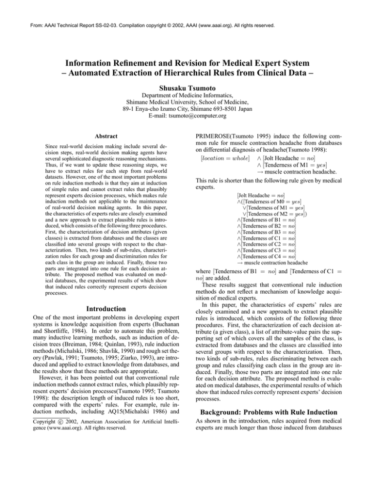
PRIMEROSE(Tsumoto 1995) induce the following common rule for muscle contraction headache from databases
on differential diagnosis of headache(Tsumoto 1998):
[location = whole] ∧ [Jolt Headache = no]
∧ [Tenderness of M1 = yes]
→ muscle contraction headache.
This rule is shorter than the following rule given by medical
experts.
[Jolt Headache = no]
∧([Tenderness of M0 = yes]
∨[Tenderness of M1 = yes]
∨[Tenderness of M2 = yes])
∧[Tenderness of B1 = no]
∧[Tenderness of B2 = no]
∧[Tenderness of B3 = no]
∧[Tenderness of C1 = no]
∧[Tenderness of C2 = no]
∧[Tenderness of C3 = no]
∧[Tenderness of C4 = no]
→ muscle contraction headache
where [Tenderness of B1 = no] and [Tenderness of C1 =
no] are added.
These results suggest that conventional rule induction
methods do not reflect a mechanism of knowledge acquisition of medical experts.
In this paper, the characteristics of experts’ rules are
closely examined and a new approach to extract plausible
rules is introduced, which consists of the following three
procedures. First, the characterization of each decision attribute (a given class), a list of attribute-value pairs the supporting set of which covers all the samples of the class, is
extracted from databases and the classes are classified into
several groups with respect to the characterization. Then,
two kinds of sub-rules, rules discriminating between each
group and rules classifying each class in the group are induced. Finally, those two parts are integrated into one rule
for each decision attribute. The proposed method is evaluated on medical databases, the experimental results of which
show that induced rules correctly represent experts’ decision
processes.
Background: Problems with Rule Induction
As shown in the introduction, rules acquired from medical
experts are much longer than those induced from databases
the decision attributes of which are given by the same experts. This is because rule induction methods generally
search for shorter rules, compared with decision tree induction. In the case of decision tree induction, the induced trees
are sometimes too deep and in order for the trees to be learningful, pruning and examination by experts are required.
One of the main reasons why rules are short and decision
trees are sometimes long is that these patterns are generated
only by one criteria, such as high accuracy or high information gain. The comparative study in this section suggests
that experts should acquire rules not only by one criteria but
by the usage of several measures. Those characteristics of
medical experts’ rules are fully examined not by comparing
between those rules for the same class, but by comparing
experts’ rules with those for another class. For example, a
classification rule for muscle contraction headache is given
by:
[Jolt Headache = no]
∧([Tenderness of M0 = yes]
∨[Tenderness of M1 = yes]
∨[Tenderness of M2 = yes])
∧[Tenderness of B1 = no]
∧[Tenderness of B2 = no]
∧[Tenderness of B3 = no]
∧[Tenderness of C1 = no]
∧[Tenderness of C2 = no]
∧[Tenderness of C3 = no]
∧[Tenderness of C4 = no]
→ muscle contraction headache
This rule is very similar to the following classification rule
for disease of cervical spine:
[Jolt Headache = no]
∧([Tenderness of M0 = yes]
∨[Tenderness of M1 = yes]
∨[Tenderness of M2 = yes])
∧([Tenderness of B1 = yes]
∨[Tenderness of B2 = yes]
∨[Tenderness of B3 = yes]
∨[Tenderness of C1 = yes]
∨[Tenderness of C2 = yes]
∨[Tenderness of C3 = yes]
∨[Tenderness of C4 = yes])
→ disease of cervical spine
The differences between these two rules are attribute-value
pairs, from tenderness of B1 to C4. Thus, these two rules
can be simplified into the following form:
a1 ∧ A2 ∧ ¬A3
a1 ∧ A2 ∧ A3
→
→
muscle contraction headache
disease of cervical spine
The first two terms and the third one represent different
reasoning. The first and second term a1 and A2 are used
to differentiate muscle contraction headache and disease of
cervical spine from other diseases. The third term A3 is used
to make a differential diagnosis between these two diseases.
Thus, medical experts firstly selects several diagnostic candidates, which are very similar to each other, from many
Table 1: An Example of Database
age
loc nat prod nau M1
1 50...59 occ per
no
no yes
2 40...49 who per
no
no yes
3 40...49
lat
thr
yes
yes no
4 40...49 who thr
yes
yes no
5 40...49 who rad
no
no yes
6 50...59 who per
no
yes yes
D EFINITIONS: loc: location, nat: nature, prod:
prodrome, nau: nausea, M1: tenderness of M1,
who: whole, occ: occular, lat: lateral, per:
persistent, thr: throbbing, rad: radiating,
m.c.h.: muscle contraction headache,
migra: migraine, psycho: psychological pain,
class
m.c.h.
m.c.h.
migra
migra
m.c.h.
psycho
diseases and then make a final diagnosis from those candidates. In the next section, a new approach for inducing the
above rules is introduced.
Rough Set Theory and Probabilistic Rules
Rough Set Notations
In the following sections, we use the following notations introduced by Skowron and Grzymala-Busse(1994), which are
based on rough set theory(Pawlak, 1991). These notations
are illustrated by a small database shown in Table 1, collecting the patients who complained of headache.
Let U denote a nonempty, finite set called the universe
and A denote a nonempty, finite set of attributes, i.e., a :
U → Va for a ∈ A, where Va is called the domain of a,
respectively.Then, a decision table is defined as an information system, A = (U, A ∪ {d}). For example, Table 1 is
an information system with U = {1, 2, 3, 4, 5, 6} and A =
{age, location, nature, prodrome, nausea, M 1} and d =
class.
For location ∈ A, Vlocation is defined as
{occular, lateral, whole}.
The atomic formulae over B ⊆ A∪{d} and V are expressions of the form [a = v], called descriptors over B, where
a ∈ B and v ∈ Va . The set F (B, V ) of formulas over
B is the least set containing all atomic formulas over B and
closed with respect to disjunction, conjunction and negation.
For example, [location = occular] is a descriptor of B.
For each f ∈ F (B, V ), fA denote the meaning of f in
A, i.e., the set of all objects in U with property f , defined
inductively as follows.
1. If f is of the form [a = v] then, fA = {s ∈ U |a(s) = v}
2. (f ∧g)A = fA ∩gA ; (f ∨g)A = fA ∨gA ; (¬f )A = U −fa
For example, f = [location = whole] and fA =
{2, 4, 5, 6}. As an example of a conjunctive formula, g =
[location = whole] ∧ [nausea = no] is a descriptor of U
and fA is equal to glocation,nausea = {2, 5}.
By the use of the framework above, classification accuracy and coverage, or true positive rate is defined as follows.
Definition 1
Let R and D denote a formula in F (B, V ) and a set of objects which belong to a decision d. Classification accuracy
and coverage(true positive rate) for R → d is defined as:
αR (D) =
κR (D) =
|RA ∩ D|
(= P (D|R)), and
|RA |
|RA ∩ D|
(= P (R|D)),
|D|
where |S|, αR (D), κR (D) and P(S) denote the cardinality
of a set S, a classification accuracy of R as to classification
of D and coverage (a true positive rate of R to D), and
probability of S, respectively.
In the above example, when R and D are set to [nau =
1] and [class = migraine], αR (D) = 2/3 = 0.67 and
κR (D) = 2/2 = 1.0.
It is notable that αR (D) measures the degree of the sufficiency of a proposition, R → D, and that κR (D) measures
the degree of its necessity. For example, if αR (D) is equal
to 1.0, then R → D is true. On the other hand, if κR (D) is
equal to 1.0, then D → R is true. Thus, if both measures are
1.0, then R ↔ D.
Probabilistic Rules
According to the definitions, probabilistic rules with high
accuracy and coverage are defined as:
α,κ
R→d
s.t.
R = ∨i Ri = ∨ ∧j [aj = vk ],
αRi (D) ≥ δα and κRi (D) ≥ δκ ,
where δα and δκ denote given thresholds for accuracy and
coverage, respectively. For the above example shown in Table 1, probabilistic rules for m.c.h. are given as follows:
[M 1 = yes]
[nau = no]
→ m.c.h.
→ m.c.h.
α = 3/4 = 0.75, κ = 1.0,
α = 3/3 = 1.0, κ = 1.0,
where δα and δκ are set to 0.75 and 0.5, respectively.
Characterization Sets
In order to model medical reasoning, a statistical measure,
coverage plays an important role in modeling, which is a
conditional probability of a condition (R) under the decision
D(P(R—D)). Let us define a characterization set of D, denoted by L(D) as a set, each element of which is an elementary attribute-value pair R with coverage being larger than a
given threshold, δκ . That is,
Lδκ = {[ai = vj ]|κ[ai =vj ] (D) ≥ δκ
Then, three types of relations between characterization sets
can be defined as follows:
Independent type: Lδκ (Di ) ∩ Lδκ (Dj ) = φ,
Boundary type:
Lδκ (Di ) ∩ L(Dj )δκ 6= φ, and
Positive type:
Lδκ (Di ) ⊆ Lδκ (Dj ).
All three definitions correspond to the negative region,
boundary region, and positive region[4], respectively, if a set
of the whole elementary attribute-value pairs will be taken as
the universe of discourse. For the above example in Table 1,
let D1 and D2 be m.c.h. and migraine and let the threshold
of the coverage is larger than 0.6. Then, since
L0.6 (m.c.h.) =
{[age = 40 − 49],
[location = whole],
[nature = persistent],
[prodrome = no],
[nausea = no], [M 1 = yes]},
L0.6 (migraine) = {[age = 40 − 49],
[nature = throbbing],
[nausea = yes], [M 1 = no]},
the relation between m.c.h. and migraine is boundary type when the threshold is set to 0.6.
Thus,
the factors that contribute to differential diagnosis between these two are: [location = whole], [nature =
persistent], [nature = throbbing], [prodrome =
no], [nausea = yes], [nausea = no], [M 1 = yes], [M 1 =
no]. In these pairs, three attributes: nausea and M1 are very
important. On the other hand, let D1 and D2 be m.c.h. and
psycho and let the threshold of the coverage is larger than
0.6. Then, since
L0.6 (psycho) = {[age = 50 − 59],
[location = whole],
[nature = persistent],
[prodrome = no],
[nausea = yes], [M 1 = yes]},
the relation between m.c.h. and psycho is also boundary.
Thus, in the case of Table 1, age, nausea and M1 are very
important factors for differential diagnosis. This relation is
dependent on the value of the threshold. If the threshold is
set up to 1.0, the characterization sets are:
L1.0 (m.c.h.) =
{[prodrome = no],
[nausea = no],
[M 1 = yes]},
L1.0 (migraine) = {[age = 40 − 49],
[nature = throbbing],
[nausea = yes],
[M 1 = no]},
L1.0 (psycho) =
{[age = 50 − 59],
[location = whole],
[nature = persistent],
[prodrome = no],
[nausea = yes],
[M 1 = yes]},
Although their contents have been changed, the relations
among three diseases are still boundary and still age, nausea
and M1 are important factors. However, it is notable that the
differences between characterization are much clearer.
According to the rules acquired from medical experts,
medical differential diagnosis is a focusing mechanism:
first, medical experts focus on some general category of diseases, such as vascular or muscular headache. After excluding the possibility of other categories, medical experts
proceed into the further differential diagnosis between diseases within a general category. In this type of reasoning,
subcategory type of characterization is the most important
one. However, since medical knowledge has some degree
of uncertainty, boundary type with high overlapped region
may have to be treated like subcategory type. To check this
boundary type, we use rough inclusion measure defined below.
Rough Inclusion
In order to measure the similarity between classes with respect to characterization, we introduce a rough inclusion
measure µ, which is defined as follows.
T
|S T |
µ(S, T ) =
.
|S|
It is notable that if S ⊆ T , then µ(S, T ) = 1.0, which shows
that this relation extends subset and superset relations. This
measure is introduced by Polkowski and Skowron (1996) in
their study on rough mereology. Whereas rough mereology
firstly applies to distributed information systems, its essential idea is rough inclusion: Rough inclusion focuses on setinclusion to characterize a hierarchical structure based on a
relation between a subset and superset. Thus, application of
rough inclusion to capturing the relations between classes
is equivalent to constructing rough hierarchical structure between classes, which is also closely related with information
granulation proposed by Zadeh(1997). Let us illustrate how
this measure is applied to hierarchical rule induction by using Table 1. When the threshold for the coverage is set to
0.6,
µ(L0.6 (m.c.h.), L0.6 (migraine)) = 16
µ(L0.6 (m.c.h.), L0.6 (psycho)) = 46 = 23
µ(L0.6 (migraine), L0.6 (psycho)) = 14
These values show that the characterization set of m.c.h. is
closer to that of psycho than that of migraine. When the
threshold is set to 1.0,
µ(L1.0 (m.c.h.), L1.0 (migraine)) = 0
µ(L1.0 (m.c.h.), L1.0 (psycho)) = 23
µ(L1.0 (migraine), L1.0 (psycho)) = 14
These values also show that the characterization of m.c.h.
is closer to that of psycho. Therefore, if the threshold for
rough inclusion is set to 0.6, the characterization set of
m.c.h. is roughly included by that of psycho. On the other
hand, the characterization set of migraine is independent of
those of m.c.h. and psycho. Thus, the differential diagnosis process consists of two process: the first process should
discriminate between migraine and the group of m.c.h. and
psycho. Then, the second process discriminate between
m.c.h and psycho. This means that the discrimination rule of
m.c.h. is composed of (discrimination between migraine and
the group)+ (discrimination between m.c.h. and psycho). In
the case of L0.6, since the intersection of the characerization
set of m.c.h and psycho is {[location = whole], [nature =
persistent], [prodrome = no], [M 1 = yes]}, and the differences in attributes between this group and migraine is nature, M1. So, one of the candidates of discrimination rule
is
[nature = throbbing] ∧ [M 1 = no] → migraine
The second discrimination rule is derived from the difference between the characterizaton set of m.c.h. and psycho:
So, one of the candidate of the second discrimination rule is:
[age = 40 − 49] → m.c.h. or [nausea = no] → m.c.h.
Combining these two rules, we can obtain a diagnostic rule
for m.c.h as:
¬([nature = throbbing] ∧ [M 1 = no])
∧[age = 40 − 49] → m.c.h.
In the case when the threshold is set to 1.0, since the intersection of the characerization set of m.c.h and psycho is
[prodrome = no], [M 1 = yes], and the differences in attributes between this group and migraine is M1. So, one
of the candidates of discrimination rule is [M 1 = no] →
migraine. The second discrimination rule is derived from
the difference between the characterizaton set of m.c.h. and
psycho: So, one of the candidate of the second discrimination rule is: [nausea = no] → m.c.h. Combining these two
rules, we can obtain a diagnostic rule for m.c.h as:
¬([M 1 = no]) ∧ [nausea = no] → m.c.h.
Rule Induction
Rule induction(Fig 1.) consists of the following three procedures. First, the characterization of each given class, a
list of attribute-value pairs the supporting set of which covers all the samples of the class, is extracted from databases
and the classes are classified into several groups with respect to the characterization. Then, two kinds of sub-rules,
rules discriminating between each group and rules classifying each class in the group are induced(Fig 2). Finally, those
two parts are integrated into one rule for each decision attribute(Fig 3).1
Example
Let us illustrate how the introduced algorithm works by using a small database in Table 1. For simplicity, two thresholds δα and δµ are set to 1.0, which means that only deterministic rules should be induced and that only subset and
superset relations should be considered for grouping classes.
After the first and second step, the following three sets
will be obtained: L(m.c.h.) = {[prod = no], [M 1 =
yes]}, L(migra) = {[age = 40...49], [nat =
who], [prod = yes], [nau = yes], [M 1 = no]}, and
L(psycho) = {[age = 50...59], [loc = who], [nat =
per], [prod = no], [nau = no], [M 1 = yes]}.
Thus, since a relation L(psycho) ⊂ L(m.c.h.) holds
(i.e.,µ(L(m.c.h.), L(psycho)) = 1.0), a new decision attribute is D1 = {m.c.h., psycho} and D2 = {migra}, and
a partition P = {D1 , D2 } is obtained. From this partition,
two decision tables will be generated, as shown in Table 2
and Table 3 in the fifth step.
In the sixth step, classification rules for D1 and D2 are
induced from Table 2. For example, the following rules are
obtained for D1 .
1
This method is an extension of PRIMEROSE4 reported in
(Tsumoto, 1998b). In the former paper, only rigid set-inclusion
relations are considered for grouping; on the other hand, roughinclusion relations are introduced in this approach. Recent empirical comparison between set-inclusion method and rough-inclusion
method shows that the latter approach outperforms the former one.
procedure Rule Induction (T otal P rocess);
var
i : integer; M, L, R : List;
LD : List; /* A list of all classes */
begin
Calculate αR (Di ) and κR (Di )
for each elementary relation R and each class Di ;
Make a list L(Di ) = {R|κR (D) = 1.0})
for each class Di ;
while (LD 6= φ) do
begin
Di := f irst(LD ); M := LD − Di ;
while (M 6= φ) do
begin
Dj := f irst(M );
if (µ(L(Dj ), L(Di )) ≤ δµ )
then L2 (Di ) := L2 (Di ) + {Dj };
M := M − Dj ;
end
Make a new decision attribute Di0 for L2 (Di );
LD := LD − Di ;
end
Construct a new table (T2 (Di ))for L2 (Di ).
Construct a new table(T (Di0 ))
for each decision attribute Di0 ;
Induce classification rules R2 for each L2 (D);
/* Fig.2 */
Store Rules into a List R(D)
Induce classification rules Rd
0
for each/*DFig.2
in T*/
(D0 );
Store Rules into a List R(D0 )(= R(L2 (Di )))
Integrate R2 and Rd into a rule RD ; /* Fig.3 */
end {Rule Induction };
procedure Induction of Classif ication Rules;
var
i : integer; M, Li : List;
begin
L1 := Ler ; /* Ler : List of Elementary Relations */
i := 1; M := {};
for i := 1 to n do /* n: Total number of attributes */
begin
while ( Li 6= {} ) do
begin
Select one pair R = ∧[ai = vj ] from Li ;
Li := Li − {R};
if (αR (D) ≥ δα ) and (κR (D) ≥ δκ )
then do Sir := Sir + {R};
/* Include R as Inclusive Rule */
else M := M + {R};
end
Li+1 := (A list of the whole combination of
the conjunction formulae in M );
end
end {Induction of Classif ication Rules };
Figure 2: An Algorithm for Classification Rules
1
2
3
4
5
6
Table 2: A Table for a New Partition P
age
loc nat prod nau M1
50...59 occ per
0
0
1
40...49 who per
0
0
1
40...49
lat
thr
1
1
0
40...49 who thr
1
1
0
40...49 who rad
0
0
1
50...59 who per
0
1
1
class
D1
D1
D2
D2
D1
D1
Figure 1: An Algorithm for Rule Induction
[M 1 = yes]
→ D1
[prod = no]
→ D1
[nau = no]
→ D1
[nat = per]
→ D1
[loc = who]
→ D1
[age = 50...59]
→ D1
α = 1.0, κ = 1.0,
supported by {1,2,5,6}
α = 1.0, κ = 1.0,
supported by {1,2,5,6}
α = 1.0, κ = 0.75,
supported by {1,2,5}
α = 1.0, κ = 0.75,
supported by {1,2,6}
α = 1.0, κ = 0.75,
supported by {2,5,6}
α = 1.0, κ = 0.5,
supported by {2,6}
[nau = no] → m.c.h. and [age = 40...49] → m.c.h. have
a supporting set which is a subset of {1,2,5,6}. Thus, the
following rules are obtained:
[M 1 = yes] & [nau=no] → m.c.h.
α = 1.0, κ = 1.0, supported by {1,2,5}
[M 1 = yes] & [age=40...49] → m.c.h.
α = 1.0, κ = 0.67, supported by {2,5}
Experimental Results
The above rule induction algorithm is implemented in
PRIMEROSE4.5 (Probabilistic Rule Induction Method
In the seventh step, classification rules for m.c.h. and
psycho are induced from Table 3. For example, the following rules are obtained from m.c.h..
[nau = no]
[age = 40...49]
→ m.c.h.
→ m.c.h.
α = 1.0, κ = 1.0,
supported by {1,2,5}
α = 1.0, κ = 0.67,
supported by {2,5}
In the eighth step, these two kinds of rules are integrated in the following way. Rule [M 1 = yes] → D1 ,
Table 3: A Table for D1
1
2
5
6
age
50...59
40...49
40...49
50...59
loc
occ
who
who
who
nat
per
per
rad
per
prod
0
0
0
0
nau
0
0
0
1
M1
1
1
1
1
class
m.c.h.
m.c.h.
m.c.h.
psycho
procedure Rule Integration;
var
i : integer; M, L2 : List;
R(Di ) : List; /* A list of rules for Di */
LD : List; /* A list of all classes */
begin
while(LD 6= φ) do
begin
Di := f irst(LD ); M := L2 (Di );
Select one rule R0 → Di0 from R(L2 (Di )).
while (M 6= φ) do
begin
Dj := f irst(M );
Select one rule R → dj for Dj ;
Integrate two rules: R ∧ R0 → dj .
M := M − {Dj };
end
LD := LD − Di ;
end
end {Rule Combination}
Figure 3: An Algorithm for Rule Integration
based on Rough Sets Ver 4.5), 2 and was applied to
databases on differential diagnosis of headache, whose training samples consist of 1477 samples, 20 classes and 20 attributes.
This system was compared with PRIMEROSE4,
PRIMEROSE, C4.5, CN2 (Clark,1989), AQ15 and k-NN
(Aha, 1991) 3 with respect to the following points: length of
rules, similarities between induced rules and expert’s rules
and performance of rules.
In this experiment, length was measured by the number
of attribute-value pairs used in an induced rule and Jaccard’s
coefficient was adopted as a similarity measure (Everitt,
1996). Concerning the performance of rules, ten-fold crossvalidation was applied to estimate classification accuracy.
Table 4 shows the experimental results, which suggest that
PRIMEROSE4.5 outperforms PRIMEROSE4(set-inclusion
approach) and the other four rule induction methods and induces rules very similar to medical experts’ ones.
Discussion
Focusing Mechanism
One of the most interesting features in medical reasoning
is that medical experts make a differential diagnosis based
on focusing mechanisms: with several inputs, they eluminate some candidates and proceed into further steps. In this
elimination, our empirical results suggest that grouping of
diseases are very important to realize automated acquisition of medical knowledge from clinical databases. Readers
may say that conceptual clustering or nearest neighborhood
2
The program is implemented by using SWI-prolog(1995) on
Sparc Station 20.
3
The most optimal k for each domain is attached to Table 4.
methods(k-NN) will be useful for grouping. However, those
two methods are based on classification accuracy, that is,
they induce grouping of diseases, whose rules are of high
accuracy. Their weak point is that they do not reflect medical reasoning: focusing mechanisms of medical experts are
chiefly based not on classification accuracy, but on coverage.
Thus, we focus on the role of coverage in focusing mechanisms and propose an algorithm on grouping of diseases by
using this measure. The above experiments show that rule
induction with this grouping generates rules, which are similar to medical experts’ rules and they suggest that our proposed method should capture medical experts’ reasoning.
Precision for Probabilistic Rules
In the above experiments, the thresholds δα and δκ for selection of inclusive rules were set to 0.75 and 0.5, respectively. Although this precision contributes to the reduction of computational complexity, this methodology, which
gives a threshold in a static way, causes a serious problem. For example, there exists a case when the accuracy
for the first, the second, and the third candidate is 0.5,
0.49, and 0.01, whereas accuracy for other classes is almost
equal to 0. Formally, provided an attribute-value pair, R,
the following equations hold: αR (D1 ) = 0.5, αR (D2 ) =
0.49, αR (D3 ) = 0.01, and αR (Di ) ≈ 0(i = 4, · · · , 10).
Then, both of the first and the second candidates should be
suspected because those accuracies are very close, compared
with the accuracy for the third and other classes. However,
if a threshold is statically set to 0.5, then this pair is not
included in positive rules for D2 . In this way, a threshold
should be determined dynamically for each attribute-value
pair. In the above example, an attribute-value pair should be
included in positive rules of D1 and D2 .
From discussion with domain experts, it is found that this
type of reasoning is very natural, which may contribute to
the differences between induced rules and the ones acquired
from medical experts. Thus, even in a learning algorithm,
comparison between the whole given classes should be included in order to realize more plausible reasoning strategy.
Unfortunately, since the proposed algorithm runs for each
disease independently, the above type of reasoning cannot
be incorporated in a natural manner, which causes computational complexity to be higher. It is our future work to
develop such interacting process in the learning algorithm.
Generality of the Proposed Method
One major character of medical reasoning is that medical
experts finally select one or two diagnostic candidates from
many diseases, called focusing mechanism. For example, in
differential diagnosis of headache, experts choose one from
about 60 diseases. The proposed method models induction
of rules which incorporates this mechanism, whose experimental evaluation show that induced rules correctly represent medical experts’ rules.
This focusing mechanism is not only specific to medical
domain. In a domain in which a few diagnostic conclusions
should be selected from many candiates, this mechanism
can be applied. For example, fault diagnosis of complicated
electronic devices should focus on which components will
Table 4: Experimental Results
Method
Length
Similarity
Accuracy
Headache
PRIMEROSE4.5
8.8 ± 0.27
0.95 ± 0.08
95.2 ± 2.7%
PRIMEROSE4.0
8.6 ± 0.27
0.93 ± 0.08
93.3 ± 2.7%
Experts
9.1 ± 0.33
1.00 ± 0.00
98.0 ± 1.9%
PRIMEROSE
5.3 ± 0.35
0.54 ± 0.05
88.3 ± 3.6%
C4.5
4.9 ± 0.39
0.53 ± 0.10
85.8 ± 1.9%
CN2
4.8 ± 0.34
0.51 ± 0.08
87.0 ± 3.1%
AQ15
4.7 ± 0.35
0.51 ± 0.09
86.2 ± 2.9%
k-NN (7)
6.7 ± 0.25
0.61 ± 0.09
88.2 ± 1.5%
k-NN (i) shows the value of i which gives the highest performance in k (1 ≤ k ≤ 20).
cause a functional problem: the more complicated devices
are, the more sophisticated focusing mechanism is required.
In such domain, proposed rule induction method will be useful to induce correct rules from datasets.
Conclusion
In this paper, the characteristics of experts’ rules are closely
examined, whose empirical results suggest that grouping of
diseases are very important to realize automated acquisition of medical knowledge from clinical databases. Thus,
we focus on the role of coverage in focusing mechanisms
and propose an algorithm on grouping of diseases by using
this measure. The above experiments show that rule induction with this grouping generates rules, which are similar
to medical experts’ rules and they suggest that our proposed
method should capture medical experts’ reasoning. The proposed method was evaluated on three medical databases, the
experimental results of which show that induced rules correctly represent experts’ decision processes.
Acknowledgments
This work was supported by the Grant-in-Aid for Scientific
Research on Priority Areas(B) (No.759) ”Implementation of
Active Mining in the Era of Information Flood” by the Ministry of Education, Science, Culture, Science and Technology of Japan.
References
Agrawal, R., Imielinski, T., and Swami, A., Mining association rules between sets of items in large databases, in Proceedings of the 1993 International Conference on Management of Data (SIGMOD 93), pp. 207-216, 1993.
Aha, D. W., Kibler, D., and Albert, M. K., Instance-based
learning algorithm. Machine Learning, 6, 37-66, 1991.
Breiman, L., Freidman, J., Olshen, R., and Stone, C., Classification And Regression Trees, Wadsworth International
Group, Belmont, 1984.
Buchnan, B. G. and Shortliffe, E. H., Rule-Based Expert
Systems, Addison-Wesley, New York, 1984.
Clark, P. and Niblett, T., The CN2 Induction Algorithm. Machine Learning, 3, 261-283, 1989.
Everitt, B. S., Cluster Analysis, 3rd Edition, John Wiley &
Son, London, 1996.
Michalski, R. S., Mozetic, I., Hong, J., and Lavrac, N., The
Multi-Purpose Incremental Learning System AQ15 and its
Testing Application to Three Medical Domains, in Proceedings of the fifth National Conference on Artificial Intelligence, 1041-1045, AAAI Press, Menlo Park, 1986.
Pawlak, Z., Rough Sets. Kluwer Academic Publishers, Dordrecht, 1991.
Polkowski, L. and Skowron, A.: Rough mereology: a new
paradigm for approximate reasoning. Intern. J. Approx.
Reasoning 15, 333–365, 1996.
Quinlan, J.R., C4.5 - Programs for Machine Learning, Morgan Kaufmann, Palo Alto, 1993.
Shavlik, J. W. and Dietterich, T.G., (eds.) Readings in Machine Learning, Morgan Kaufmann, Palo Alto, 1990.
Skowron, A. and Grzymala-Busse, J. From rough set theory to evidence theory. In: Yager, R., Fedrizzi, M. and
Kacprzyk, J.(eds.) Advances in the Dempster-Shafer Theory
of Evidence, pp.193-236, John Wiley & Sons, New York,
1994.
SWI-Prolog Version 2.0.9 Manual, University of Amsterdam, 1995.
Tsumoto, S. and Tanaka, H., PRIMEROSE: Probabilistic
Rule Induction Method based on Rough Sets and Resampling Methods. Computational Intelligence, 11, 389-405,
1995.
Tsumoto, S., Automated Induction of Medical Expert System Rules from Clinical Databases based on Rough Set Theory. Information Sciences 112, 67-84, 1998.
Tsumoto, S. Extraction of Experts’ Decision Rules from
Clinical Databases using Rough Set Model Intelligent Data
Analysis, 2(3), 1998.
Zadeh, L.A., Toward a theory of fuzzy information granulation and its certainty in human reasoning and fuzzy logic.
Fuzzy Sets and Systems 90, 111-127, 1997.
Ziarko, W., Variable Precision Rough Set Model. Journal of
Computer and System Sciences. 46, 39-59, 1993.