From: AAAI Technical Report SS-94-06. Compilation copyright © 1994, AAAI (www.aaai.org). All rights reserved.
Decison-Theoretic
Peter
Refinement Planning
Abstraction
Haddawy
* Meliani
using
Inheritance
Suwandi
Department of Electrical
Engineering and Computer Science
University of Wisconsin-Milwaukee
PO Box 784
Milwaukee, WI 53201
1
el
1
Introduction
Pll
Givena probabilistic modelof the world and of available
actions and a utility function representing the planner’s
objectives wewish to find the plan that maximizesexpected utility. Finding the optimal plan requires comparing the expectedutilities of all possible plans. Doing
this explicitly wouldbe computationallyprohibitive in
all but the smallest of domains.Thuswemust find a way
to comparepartial plans in such a waythat wecan eliminate somepartial plans before fully elaborating them.
Suchcomparisonsrequire a definition of partial plan that
allows us to determinethat all completionsof one plan
are less preferred than all completionsof another. We
achieve such a definition of partial plan by structuring
actions into an abstraction hierarchy and by restricting
the planner to using only refinement operators. Apartial
plan is then a plan in whichsomeof the actions are abstract. Anabstract plan’s outcomesare sets of outcomes
of moreconcrete plans. Since different probability and
utility values maybe associated with each specific outcome,in general a probability range and a utility range
will be associated with each abstract outcome.Thusthe
expectedutility of an abstract plan is represented by an
interval, whichincludes the expectedutilities of all possible instantiations of that abstract plan. Refining the
plan, i.e. instantiating on of its actions, tends to narrow
the interval. Whenthe expectedutility intervals of two
plans do not overlap, the one with the lower interval can
be eliminated.
Wepresent a methodfor abstracting probabilistic conditionM actions and we show howto computeexpected
utility boundsfor plans containing such abstract actions.
Wepresent a planning algorithm that searches through
the space of possible plans by building abstract plans,
comparingthem, and refining only those that might be
refinable to the optimal plan. The algorithm is guaranteed to find the optimal plan and with an appropriate
abstraction hierarchy has a complexitywhichis exponentially better than that of exhaustive enumeration. The
planning algorithm has been implementedas the DRIPS
decision-theoretic refinement planning system. The sys*Thisworkwasinspiredby discussionswithSteveHanks.
Manonton
Butarbutar
performed
the complexityanalysis of
the algorithm.This workwaspartially supportedby NSF
grant #IRI-9207262.
Pl2
C12
Cl
m
plm
A
Pkl
ekl
ek
2
Pk2
~o
eko
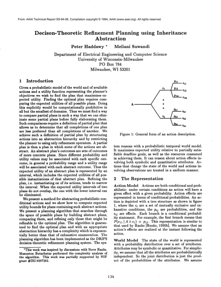
Figure 1: Generalform of an action description.
temreasons witha probabilistic temporal world model.
It maximizes
expectedutility relative to partially satisfiable deadline goals, as well as the resources consumed
in achievingthem. It can reason about action effects involving both symbolic and quantitative attributes. Actions that changethe state of the world and actions involving observations are treated in a uniformmanner.
2
The Representation
Action ModelActions are both conditional and probabilistic: under certain conditions an action will have a
given effect with a given probability. Actioneffects are
representedin terms of conditional probabilities. Anaction is depicted with a tree structure as shownin figure
1, wherethe ci are a set of mutually exclusive and exhaustive conditions, the Pij are probabilities, and the
eij are effects. Eachbranch is a conditional probability statement. For example,the first branch meansthat
P(e11[ A A el) = Pro. This representation is similar to
that used by Hanks[Hanks, 1990b]. Weassumethat an
action’s effects are realized at the instant followingthe
action.
World Model The state of the world is represented
with a probability distribution
over a set of attributes.
Attributes may be symbolic or quantitative.
For simplicity, we assume that all the attributes are probabilistically
independent. So the joint distribution
is just the product of the probabilities
of the attributes.
We assume
134
dM
l-
2
85
tons
165 time
UR
1-
2.5
A
Figure 3: Abstracting probabilistic
conditional actions.
4.5f~el
Figure 2: Specification of delivery utility function.
that changes to the world are limited to those effects explicitly described in the agent’s action descriptions. We
do not allow for exogenous events.
Utility Model Weuse the goal-directed utility model
for deadline goals described in [Haddawy and Hanks,
1992, Haddawy and Hanks, 1993]. A deadline goal,
such as delivering two tons of tomatoes to the warehouse within 85 minutes, is considered to consist of a
temporal and an atemporal component. The atemporal component indicates what is to be achieved and the
temporal componentindicates when it is to be achieved.
Our exampledeadline goal could be partially satisfied in
two ways: we can partially satisfy the atemporal component by delivering less than two tons of tomatoes and we
can partially satisfy the temporal component by making
our delivery after the deadline. Of course, we can partially satisfy both components by making several small
deliveries both before and after the deadline. A utility
function relative to such a goal is specified in terms of a
degree of satisfaction function for the atemporal component (DSA) and a temporal coefficient
(CT). The
function indicates to what degree the atemporal component is satisfied at a time in a chronicle and the temporal coefficient is a discount factor that penalizes the
planning agent for missing the deadline. The utility of
a chronicle relative to a goal is computed by combining
the two functions. This is done by summingthe DSAat
the deadline with the changes in DSAafter the deadline,
weighted by the temporal coefficient. Werepresent the
costs associated with attempting to achieve a goal with
a residual utility function (JR. Assumingthat the goal
and residuM utility are independent, the overall utility
of a chronicle is the sumof the goal and residual utilities.
Figure 2 shows some possible utility functions for our
tomato delivery example. If we only obtain benefit from
having all tomatoes delivered, the DSAfunction would
be a step function with value zero below two tons and
value one above two tons. If we can obtain benefit from
deliveries that miss the deadline we might represent the
temporal coefficient as a linear function that has value
one at 85 minutes and value zero at say 165 minutes.
If our only cost is the amount of fuel consumed then
the residual utility might be a linear function with value
one at 2.5 gallons consumption and value zero at 4.5
gallons. If a unit of goal utility is worth .02 units of
residual utility, we could represent the overall utility as
U(c) = UG(c) + (.02)UR(c).
The Planning Task A planning problem is described
in terms of an initial state distribution, a set of action
descriptions, and a utility function. The action descriptions are organized into an abstraction/decomposition
network, which is described in section 5. A plan is a
sequence of actions. So the planning task is to find the
sequence of actions that maximizesexpected utility relative to the given probability and utility models.
3
Abstracting
Actions
135
Weextend Tenenberg’s [Tenenberg, 1991] notion of inheritance abstraction for STRIPSoperators to apply to
conditional probabilistic actions. As Tenenbergexplains
it, "the intent of using inheritance abstraction is to formalize the notion that analogous action types can be
structured together into an action class at the abstract
level characterized by the commonfeatures of all elements of the class." Thus we can plan with the abstract
action and infer properties of a plan involving any of the
instances of the abstract action.
Weabstract actions by grouping their outcomes. If
one action has an outcome el and another action has
an outcome e2 then we can produce an abstract action
with outcome E such that E is consistent with both el
and e2. Consider the two actions a and a’ shown in figure 3. Suppose we wish to produce an abstract action A
by grouping topologically corresponding branches. Then
under what conditions and with what probabilities will
effect Ell be realized? First we consider the conditions
under which it will be realized. It will certainly be realized with some probability in any world in which both
condition ct and c~ occur. It could be realized with some
probability in any world in which cl or c~ occurs. Thus
the range of worlds in which Ell is realized with some
probability is described by [cl A c~ cl V c~]. Notice that
the set of models satisfying et A c~ is a strict subset of
the set of modelssatisfying cl V c~, so the range is well
defined. Nowwe must determine with what probability
Ell is realized in such worlds. If action a is chosen as
the instantiation, it is realized with probability Pll and
if action a’ is chosen it is realized with probability P~I.
So it is realized with a probability in the range [Pll P~I].
Thus the probability that effect Ell is realized along the
first branch is at least P(el A c~). min(pll,p~l) and at
most P(Cl V c~) . max(p11,Pll
Our method of representing abstract actions is similar to that of Chrisman [1992]. He represents the uncertainty in the effects of an abstract action by using
Dempster-Shafer intervals. He derives a closed-form projection rule that works by finding the convex hull of possible poststate probability distributions. Although his
actions can include conditions, he does not show how to
abstract the conditions.
4
Evaluating
Plans
The outcome of a plan is a probability distribution over
a set of chronicles. Weneed to compute this distribution from the initial state distribution and the action
descriptions.
We make the Markovian assumption that
the conditional probabilities of an action’s effects given
the action and the conditions in its description are independent of all other conditions at the sametime or earlier
and all other previous actions. Wealso assume that the
conditions determining the effects of an action are probabilistically
independent of the action. Under these
assumptions, we can compute the outcome distribution
of an action by multiplying the conditional probabilities
describing the action effects by the probabilities of the
conditions. Projecting a plan produces a probability distribution over a future-branching tree of chronicles. In
practice, we compute the set of outcome chronicles of
a plan by starting with a set of worlds with probabilities assigned to them and by projecting the action in
each of those worlds. In each world the action produces
the resulting distribution associated with the conditions
that are true in that world. Thus if actions have probabilistic effects, as we project a plan forward the set of
worlds increases, i.e. we generate a future-branching set
of chronicles. Weneed to distinguish the separate chronicles since utility is a function of attribute values over
time.
Projecting an abstract plan will result in a set of
chronicles characterized by duration ranges and attribute ranges after each action in the plan, as well as a
range on the probability of each chronicle. In order to
compute expected utility bounds for abstract plans, we
need to be able to translate the attribute and duration
ranges into a range for the utility of the chronicle. In
order to do this we must make some assumptions con-
136
cerning the form of the DSAfunction. For quantitative
attributes we assume that DSAis a monotonic function
of the quantity. So for each outcome, either the upper
bound or the lower bound of the values corresponds to
the upper bound of the utility of the chronicle, and the
other one corresponds to the lower bound of the utility
of the chronicle. For deadline goals, achieving the goal
at the earliest time is preferred, and so has the highest
utility. Thus the maximumvalue of the utility corresponds to the lower bound of the range of time, and the
minimumvalue to the upper bound.
5
The
Planner
Wedescribe the DRIPSplanning system by demonstrating how it handles an example problem. Suppose we wish
to generate the best plan for delivering two tons of tomatoes from a farm to a warehouse within 85 minutes1 and
suppose we use the example utility function from section
2. The delivery plan will consist of driving a truck from
the depot to the farm, loading the truck, and driving the
loaded truck to the warehouse. Planning is the process
of generating this plan as well as choosing among the
various ways this plan can be realized in such a way that
expected utility is maximized. The descriptions of the
available actions are shown in Figure 4. The leaves of
the trees are labeled with the outcomes of the actions.
Deterministic actions are labeled with a single outcome.
Outcomes are described in terms of a duration, as well
as any changes in attribute values. Attributes are represented as functions of time. The variable t represents
the beginning time of the action, making the action descriptions temporally indexical.
There are two possible routes we can take from the depot to the farm: road A and road B. Road A is longer but
has no delays, while travel along road B might be delayed
due to construction. The probability that construction
is taking place is 0.2. These options are represented by
the first two action descriptions in the Figure 4.
Once at the farm we must load the truck. Wehave
two trucks at the depot to choose from: an open truck
and a closed, cushioned truck. The open truck is easy
to load, while there is an 80%chance the closed truck
can be loaded quickly and a 20%chance that loading it
will take longer. The next two diagrams in the Figure 4
depict these two actions.
Once the truck is loaded we must drive it to the warehouse. Wehave two routes to choose from: the mountain
road and the valley road. The mountain road is shorter
but bumpy. If we drive the open truck on the mountain
road, the bottom 20% of the tomatoes will be crushed.
If we drive the open truck on the valley road and the sun
is shining, the top 10%of the tomatoes will be spoiled
by the sun. This combination of options results in the
last four action descriptions in the Figure 4.
The DRIPSsystem searches for the optimal plan using
an abstraction/decomposition
network which describes
the space of possible plans and their abstractions. The
1 For simplicity of exposition our exampleincludes only
quantitative attributes but DRIPSis capable of reasoning
about symbohcattributes as well.
GoIo farmI dUrl= 30
deliver
~m~es
om~uSA
L~(t+durP=~(t>-t
]
coml~uctiou
]fua1(t+dur2)=fu~t)-l~
~10ad
&drive
track
goto
faun
1
//
~
%
%
~adA
S
.,sss~sssp
¯
madB Ioad,~
~vc
%%
"%.
%%.
load&~vc
loadoI~~ ~ivcopcnlmcklmlclomi_._~~wclomtt~ck
lmck
to wa=homm~k
to wa~om
/ \
/ \
\
/
//
\
/
\
\
/
%
i
t
\
I
\
on
cbivc
o!~on
~vcopm
on ddvc
closcd
on ~vcclosed
toad
mountain
mad valley
mad moum~.
~ad v~ey
Driveopentruest
on valley mid
Drive¢lm~lIru"4’ [
ou moenJa-/rmxJ
L
Drived~edtrack [
oe uUey rutd t
Figure 5: Abstraction/decomposition
Figure 4: Action descriptions for the delivery example.
networkfor this problem is shownin Figure 5. Solid links
show decompositions, while dashed links show possible
refinements. For example the task "deliver tomatoes"
is decomposedinto the sequence of the two actions "go
to farm" and "load & drive truck". The arrow between
the actions signifies temporal succession. The abstract
action "go to farm" can be realized by driving on road
A or road B. Since both elements of a decomposition
must be realized, decomposition links are ANDlinks and
since either element of an instantiation may be used,
instantiation links are ORlinks. So this network forms
an AND/ORtree.
Descriptions of the abstract actions are shownin Figure 6. A set of actions is abstracted by grouping together their outcomes into abstract outcomes which represent the range of possible outcomes of the instantiations. Care must be taken to group together similar
outcomes. For example, the "drive open truck" action is
an abstraction of "drive open truck on mountain road"
and "drive open truck on valley road." Since the single
outcome of "drive open truck on mountain road" is more
similar to the outcomeof the upper branch of "drive open
truck on valley road" than to the outcome of the lower
branch, it is grouped with the former. While similarity is fairly clear in this case, determining similarity of
outcomes with multiple attributes may not be straightforward in general. (In fact, one may wish to produce
more than one abstraction based on different similarity
measures and try each one on a given problem. One
would use the hierarchy that resulted in the most pruning for the given problem.) The outcomes of the abstract
action are now specified simply as the range of outcomes
137
network.
grouped together.
Given this representation of the planning problem, we
evaluate plans at the abstract level, eliminate suboptimal plans, and refine remaining candidate plans further.
The algorithm works as follows. The algorithm uses two
primary data structures. A queue contains all actions
that might need to be refined. A list called plans contains all candidate plans.
Procedure:
Create a plan consisting of the single top-level
action and put it in plans.
Put the action on the queue.
Until the queue is empty do:
Take the first action from the queue.
If the action does not appear in any
plans or is a concrete action, do nothing.
Else it is an abstract action, so
Until no plans contain the action do
¯ Replace a plan in which the
action appears with one plan
for every possible instantiation of the action.
¯ Replace the instantiations
with their decompositions.
¯ Compute the expected utility range of each new plan.
¯ Remove suboptimal plans
from plans.
Return plans.
Eight possible plans are implicitly encoded in the abstraction/decomposition network, and we want to choose
[-’~o~tnmfion ~
(
Goto farm
Idm "45
\
ginning time of an action to be the beginning time of the
previous action plus its duration. So for examplethe fuel
consumption for chronicle Cl is computed according to
Idur8- [1530].
[ f~l(t+dura)"fuel(t)-[1/2
IF ¢vmmwaion]Ifuei(t+dur@=f~l(0-1/2
I
fuel(durs)
= fuel(O) [. 5 1]
fuel(durs + dur9) = fuel(durs)
[23]
so
Drive
open
truck
~
du~=[6090]
fuel(t+durg)= fuel(t)-[2
I
tom--deliveved(t+dexg)
= [.8.9] tons-in-truck(t)[
I
dUrg=90
~](t+~)
l fuel(t)--3
[IF -mmny]tom_delivered(t+dur9)= tons_in_truck(t)
timed
truck
I
dtwlO- [60 90]
fiml(t+durtO)
- fuel(O-[2
tom-denvefed(t+durT) - tom-i~(t)
I
I
]
fuel(durs ÷ durg) = fuel(O) [2.5 4]
Weillustrate how the utility range is computed by showing the computation for chronicle c2 of plan 791. The
computations for the other chronicles are similar. Let
UGmin and UGma~:be the lower and upper bounds on
the goal utility, respectively, and let UR,~I, and UR~a~
be the lower and upper boundson residual utility, respectively. Weminimizethe utility of the abstract chronicle
by choosing the latest delivery times and the smallest
delivery amounts and maximize the utility by choosing
the earliest delivery times and the largest amounts. So
UGma,,,(c2)= dsa(2), ct(120) = 0.5625
Figure 6: Abstract action descriptions.
UGmin(c2)= dsa(2), ct(135) = 0.375
ORmin(C2)
1o1: Go to farm ----* Load & drive open truck
time
fuel
tons
U(chron)
[90 1351
[2.5 41
[1.6 1.81
[.005.021
chron
Cl
.c2
c3
c4
[120135]
[120 1501
150
chron
Cl
c2
¢3
c4
"P2: Go to farm ----* Load & drive
time
fuel
tons
2
[85130] [2.541
2
[100145] [412.5
2
[115145] [2.5
3.5]
2
[130 160] [2.5 3.5]
[3.54]
s.5
[2.5 3.51
2
[1.6 1.8]
2
[.380.5725]
[.01 .02]
.1975
prob
[.56 1]
[0.3]
[0 .2]
[0 06]
closed truck
prob
U(chron)
[.44251.02] [.64
.8]
[.255
.8325] [.16 .2]
[.255
.635] [0.16]
[.0675 .4475] [0 .04]
Table 1: Highest level abstract plan outcomes.
theonethatmaximizes
expected
utility.
According
to
thenetwork,
thetaskofdelivering
tomatoes
is firstdecomposed
intogoingto thefarmandloading,
thendrivingthe truck.The plannerattempts
to choosean instantiation of the "go to farm" action first. Because the
utility function is a function over chronicles, the value
of a particular action in a plan depends on when in the
plan it occurs, so options can only be evaluated in the
context of an overall plan. Consequently, we combine the
"load ~ drive open truck" and the "load & drive closed
truck" actions with the "go to farm" action to obtain a
complete abstract plan that can be evaluated.
Eachabstract plan results in four chronicles (Table 1).
For example, for plan 791 we obtain these chronicles by
concatenating the "go to farm," "load open truck," and
"drive open truck" action descriptions. Doing so results
in four chronicles, since "go to farm" and "drive open
truck" each have two branches. Rather than showing the
complete chronicles, the relevant attributes of the resulting chronicles are summarized in Table 1, which shows
for each chronicle the range of times, fuel consumption,
and tons of tomatos delivered. The time refers to the
time that the delivery is made. Weassume that the
plan begins execution at time zero and we take the be-
138
= 0.25
URmax(c2)= 0.5
Since our global utility function is U(c) = UG(c)
(0.02)UR(c), we have U(c2) = [0.380 0.5725].
Using the utility and probability information in the table we can compute the expected utility bounds for each
plan. Computing a bound for a plan involves choosing
the probabilities within the given ranges that minimize
and maximize the expected utility.
We can do so by
solving a small linear programming problem in which
the objective function is the expression for the expected
utility and the constraints are the probability bounds.
For example, the upper bound for plan 791 can be computed by maximizing the objective function
¯02pl + .5725p2 + .02p3 +. 1975p4
subject to the constraints
.56_<pl <_ 1, 0_<p2_<.3,
0_<p3 <.2,
0<p4<.06,
PI+P2+P3+P4 = 1
The maximizing probabilities are
Pl ----
.56 P2 :
.3
P3 -- .08 P4 --
So the upper bound on expected utility
.06
is
(.56)(.02) + (.3)(.5725) + (.08)(.02) + (.06)(.
So for plan 791 and 792 we obtain the expected utility
ranges EU(791) = [.005 .1964] and Eu(792)- [.3673
.9825]. Since the lower bound for 792 is greater than the
upper bound for 791, we can eliminate from consideration
all possible refinements of 791 and concentrate on refining
792. So at this point we have chosen the option of using
the closed truck. By making this choice, we have pruned
away the left-hand subnetwork underneath the "load &
drive truck" node in Figure 5, resulting in pruning half
the space of possible plans from consideration.
6
"P3.1: Go to farm ~ Load closed --+ Drive closed on mt.rd.
prob
chron
time
fuel
tons
U(chron)
el
[86 100]
[2.5 3]
2
[.8275 1.02]
[.64 .8]
2
[.64 .8325]
[.16 .2]
[100 115] [2.53]
¢2
c3
115
2.5
2
,645
[0 .16]
ct
130
2.6
2
.4675
Analysis
The complexity of decision-theoretic refinement planning
is a function of two factors: the numberof plans and the
length of plans. The DRIPSapproach reduces complexity as a function of the numberof plans. Supposewe have
an abstraction/decomposition network with p actions in
each decomposition, n possible instantiations of each abstract action, and k levels of abstraction. This network
contains n(p+p2+ps+’’’+pk) possible concrete plans, which
is a huge number even for small values of n, p, and k.
For example if we have only three instantiations of each
abstract action, four actions in each decomposition, and
s4
three levels of abstraction then the network contains 3
possible concrete plans. Nowsuppose that x is the percentage of the plans remaining at each abstraction level
after pruning. For a poorly chosen hierarchy, the value of
x is 100%,i.e., none of the plans are pruned, and for an
ideally chosen hierarchy, the value of x times the number of current plans is 1, i.e., at each abstraction level
all abstract plans are pruned except one. The number
of plans (abstract and concrete ) for which the DRIPS
algorithm computes expected utility is
[0 .o4]
P3.3: Go to farm ~ Load closed ----+ Drive closed on valley rd. I
chron
time
fuel
tons
prob
U(chron)
cI
[I15 130] [3.5 4]
2
[.4425 .635]
[.64 8] I
c
2
[.255
.4475] [.16
.2]
[130145] [3.5
4]
2
3.6
2
.26
c3
146
[0 .16]
3.5
2
.0725
c
160
[0.04]
4
Table 2: Intermediate level abstract plan outcomes.
92.1.1:
chron
e
1
c3
92.1.2:
chron
ci
c2
c3
c4
Complexity
Go on A-----~Load closed---,Drive closed on mt.rd.
time
fuel
tons
prob
U(chron)
100
3
2
.8275
.8
115
3
2
.64
.2
Go on B----~Losdclosed----~Drive
closedon mt. rd.
time fuel tons U(chron)
prob
85
2.5
2
1.02
.64
.8325
.16
100 2.5
2
.645
.16
115
2.5
2
130
2.5
2
.4575
.04
Table3: Concrete
planoutcomes.
n .-{-
xn2 ..-1-
x2n3 +...
-’1- xP+P"+’"+Pk--lnp+P"+’"+Pk
¯
With maximumpruning (xn = 1) the number of plans
examined is only
We’ are left with two more actions to refine: "go to
farm" and "drive closed truck to warehouse." The planner chooses to refine the drive action. Again the instantiations involving the mountain road and the valley road
must be evaluated in the context of a complete plan.
So we compose the descriptions of the concrete actions
"drive closed on mountain road" and "drive closed on
valley road" with the descriptions of the concrete action
"load closed truck" and the abstract action "go to farm."
Table 2 summarizesthe outcomes for the two alternative
plans. Weuse this information to compute expectedutility bounds for the two alternatives:
EU(P2.1)
[.7533.9825] and EU(P2.2) = [.3683.5975]. Notice that
the EUintervals for the two plans are contained in the
EUinterval for the abstract plan of which they are a refinement. Since the lower bound for plan ~2.1 is greater
than the upper bound for plan P2.2, we can eliminate
P2.2 from consideration, pruning away two more possible concrete plans. By eliminating plan 7~2.2, we have
chosen to take the mountain road.
Finally we refine plan P2.1. Our two options are taking either road A or road B to the farm. The outcomes
of the plans incorporating these options are summarized
in table 3. Since the plans now include only concrete
actions, the attribute, probability, and utility values are
now point values. The expected utilities of the two remaining plans are EU(~O2.1.1) = .79 EU(P2.1.2) = .9075
so we choose plan P2.1.2, which is "go to farm on road B",
"load closed truck", and "drive closed truck on mountain
road". Since this is a complete concrete plan, we have
generated the plan that maximizes expected utility and
are finished.
139
n-I- xn x n-Jr (xn) 2 × n +....+ (xn) p+p2+’’’+pk-1× n =
n(p + p2 + ... + pk),
a logarithmic reduction in complexity. With no pruning
(xn = n) the number of plans examined is
n-~ n2 ~- n3 ~- . . . + np+p~+’’’+pk
which is more than the number examined by simply exhaustively enumerating all plans since we examine the
abstract plans as well as the concrete ones. But an
asymptotic analysis shows that this numberis not significantly greater than the total number of concrete plans
when the number of plans is very large. If u is the number of possible concrete plans represented in the network
then with maximump~uning the total number of plans
examined by the DRIPS algorithm is O(log(u)).
no pruning the total number of plans examined is O(u).
This is to say that using abstraction we reduce the complexity logarithmically for the best case, while we retain
the same complexity for the worst case.
7
Conclusions
and
Future
Research
Wehave presented a decision-theoretic planner that reduces the complexity of planning by using inheritance
abstraction. The planner finds the expected utilitymaximizingplan by repeatedly instantiating abstract actions, computing expected utility, and pruning suboptimal classes of plans. The system reasons with a rich
domain representation that includes time and both symbolic and numeric attributes.
The planner finds plans
to achieve partially satisfiable deadline goals. Because
the planning algorithm works by eliminating suboptimal
plans, it can be stopped at any time to obtain the current
set of possibly optimal plans.
DRIPSis intended to be a practicM planning system
for solving large real-world planning problems. To test
its usefulness, we are applying it to the problemof planning the brewing of beer. Our current domain model
contains approximately 280 possible plans and we anticipate that the final modelwill be significantly larger.
In addition to applying DRIPS to large problems,
we are interested in extending the scope of problems
that DRIPScan solve, as well as making it easier to
use. Weare currently adding the capability to plan
for partially satisfiable maintenance goals [Haddawyand
Hanks, 1993]. A maintenance goal specifies that a condition should be maintained over a period of time. Adding
this capability only requires adding the ability to compute expected utility ranges for the newutility functions.
The efficiency of DRIPSdepends on how well the abstraction hierarchy is suited to the utility function for
which a plan is being generated. In the worst case, the
algorithm performs more work than that involved in exhaustively enumerating all possible plans. Weare examining ways in which the abstraction hierarchy can be
dynamically tailored to each given utility function by
indexing off of certain characteristics of the utility function.
The DRIPSalgorithm reduces planning complexity as
a function of the number of plans by using abstraction.
Abstraction can also be used to reduce complexity as a
function of plan length. The complexity of planning under uncertainty increases exponentially as a function of
plan length because each action may have several possible outcomes and the total number of outcomes of a plan
is the product of the number of outcomes of each of its
actions. This complexity can be reduced by using a form
of abstraction in which some of the outcomes of an action are bundled together, thus reducing the branching
factor [Hanks, 1990a]. Incorporating this kind of abstraction into the DRIPSframeworkraises several interesting questions. The planner must be able to represent
both abstraction of outcomes and abstraction into action
classes at the same time. The planner must decide when
to refine the bundled outcomes of an action versus when
to refine abstract action classes.
The DRIPSplanner finds the optimal plan by searching through a static abstraction/decomposition network.
The need to completely specify the network places a large
burden on the user. Generation of task decompositions
is the problem addressed by traditional nonlinear planners. A nonlinear planner could be used to generate the
decompositions.
References
[Chrisman, 1992] L. Chrisman. Abstract probabilistic
modeling of action. In Proceedings of the First International Conferenceon Artificial Intelligence Planning Systems, pages 28-36, June 1992.
[Haddawy and Hanks, 1992] P. ttaddawy and S. Hanks.
Representations for decision-theoretic planning: Utility functions for deadline goals. In B. Nebel, C. Rich,
140
and W. Swartout, editors, Principles of Knowledge
Representation and Reasoning: Proceedings of the
Third International Conference (KRg~), pages 71-82.
Morgan Kaufmann, San Mateo, CA, 1992.
[Haddawy and Hanks, 1993] P. Haddawy and S. Hanks.
Utility models for goal-directed decision-theoretic
planners. Technical Report 93-06-04, Department
of Computer Science and Engineering, University of
Washington, June 1993. (Also submitted to Artificial
Intelligence).
[Hanks, 1990a] S. Hanks. Practical temporal projection.
In Proceedings of the Eighth National Conference on
Artificial Intelligence, pages 158-163, Boston, July
1990.
[Hanks, 1990b] S. Hanks. Projecting Plans for Uncertain Worlds. PhD thesis, Yale University, January
1990.
[Tenenberg, 1991] J.D. Tenenberg. Reasoning About
Plans, pages 213-283. Morgan Kaufmann, San Mateo, CA, 1991.