From: AAAI Technical Report SS-94-05. Compilation copyright © 1994, AAAI (www.aaai.org). All rights reserved.
Recognition Of Red Blood Cells Abnormalities Using a New Set of Closed Contour
Features
Ahmed R. Bashandy
Computer Science Department
Purdue University
West Lafayette
IN 47906
Ahmed Darwish
Samir I. Shaheen
Electronics and Communication Dept.
Electronics and Communication Dept.
Faculty Of Engineering
Faculty Of Engineering
Cairo University
Cairo University
Giza, Egypt
Giza, Egypt
A pixel will be denoted by the symbol xi or xi(m,n), where m
Abstract
represents the horizontal axis and n represents the vertical axis
Diagnosis of anemia depends upon the observation of
variations in color, shape and gray level distribution inside the A continuous contour is defined as a set of points P
Red Blood Cells (RBC's). The most important of all is the variation P = {xi(mi,ni) : |mi-mi+1|<=1, |ni-ni+1|<=1,
in the outer contour of an individual cell. In this paper, several
NOT (ni=nj and mi=mj) for i≠j, i,j=1,..,N } ......(1)
new closed contour features are presented, together with some
techniques for preprocessing and feature extraction. Preprocessing A closed contour is defined as the set of points C
includes contour extraction and run length coding of a closed C = { continuous contour , |m -m |<=1, |n -n |<=1,
N 1
N 1
contour, while features include concavity, unsymmetry and zero
NOT (n1=nN and m1=mN) i,j=1,..,N} ......(2)
crossing of slope density curve. Features are rotation, where
transformation and scale invariant in addition to being highly
N = number of points in the contour
noise tolerant. An efficient design of a decision tree is presented
3. Preprocessing
for classification.
Preprocessing includes smoothing, thresholding, contour
extraction and run-length coding of each individual cell.
1. Abnormalities of Red Blood Cells
With the inspection of a large variety of RBC's [13,14], 3.1. Smoothing
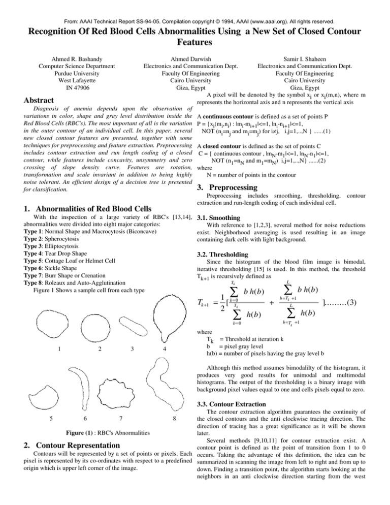
abnormalities were divided into eight major categories:
With reference to [1,2,3], several method for noise reductions
Type 1: Normal Shape and Macrocytosis (Biconcave)
exist. Neighborhood averaging is used resulting in an image
Type 2: Spherocytosis
containing dark cells with light background.
Type 3: Elliptocytosis
Type 4: Tear Drop Shape
3.2. Thresholding
Type 5: Cottage Loaf or Helmet Cell
Since the histogram of the blood film image is bimodal,
Type 6: Sickle Shape
iterative thresholding [15] is used. In this method, the threshold
Type 7: Burr Shape or Crenation
Tk+1 is recursively defined as
L
Tk
Type 8: Roleaux and Auto-Agglutination
b h( b )
Figure 1 Shows a sample cell from each type
b h( b )
Tk +1
1 ∑
= [ b =T0k
2
∑
∑
+
h( b )
b=0
1
2
3
b = Tk +1
].........(3)
L
∑
h( b )
b = T +1
k
where
Tk = Threshold at iteration k
b
= pixel gray level
h(b) = number of pixels having the gray level b
4
Although this method assumes bimodalilty of the histogram, it
produces very good results for unimodal and multimodal
histograms. The output of the thresholding is a binary image with
background pixel values equal to one and cells pixels equal to zero.
3.3. Contour Extraction
The contour extraction algorithm guarantees the continuity of
the closed contours and the anti clockwise tracing direction. The
direction of tracing has a great significance as it will be shown
Figure (1) : RBC's Abnormalities
later.
Several methods [9,10,11] for contour extraction exist. A
2. Contour Representation
contour point is defined as the point of transition from 1 to 0
Contours will be represented by a set of points or pixels. Each occurs. Taking the advantage of this definition, the idea can be
pixel is represented by its co-ordinates with respect to a predefined summarized in scanning the image from left to right and from up to
origin which is upper left corner of the image.
down. Finding a transition point, the algorithm starts looking at the
neighbors in an anti clockwise direction starting from the west
5
6
7
8
pixel. Figure (2) summarizes the algorithm. Refer to [16] for the
Using the run length code, the points inside the contour can be
complete algorithm.
used for calculation of moments of an arbitrary order. Refer to
[1,2,3,4,12] for using moments as features.
4. Features
In this section, the seven features, together with the methods of
extraction, are presented.
4.1. Minimum Bounding Rectangle (Aspect Ratio)
This is a measure of elongation. In order to find the aspect
ratio, one has to find the orientation of the shape. The orientation
angle is defined as
Figure (2) : Contour Extraction Algorithm
θ=
2 µ1,1
1
tan -1
µ 2,0 − µ 0,1
2
..... ..... . (5)
The output is a set C of points representing the closed contour where
θ
= orientation angle
for each cell in the image.
µm,n= central moments of order m,n
3.4. Run Length Coding of a closed Contour
By rotating the shape with -θ, the aspect ratio is calculated so
Run length coding of a close contour is primarily needed to
differentiate between points inside the contour and outside it. It is as to be greater than 1. A value of 1 is subtracted.
also needed for moment calculation and filling cells which is
needed to solve some problems in the contour extraction algorithm. 4.2. Unsymmetry
The property measures the uniformity of distribution of area
Although the general polygon filling algorithm [6] can be used, it
will be computationally very expensive since the number of sides inside the bounding contour. Consider figure 4.
will be very large.
Figure 4: Unsymmetric Shape
Assume that the contour is a wire, that is, there is only linear
density. The centroid (contour centroid) will be attracted to the
right direction. If, on the other hand, the contour bounds an area,
Figure (3) : Run Length Coding
the centroid (area centroid ) will tend to be on the left side, since
most of the area is concentrated in the left side. It is proved in [16]
Run length coding is the process of finding the set of horizontal that, for an arbitrary symmetric shape, the contour and area
scan lines such that all the scan lines lie completely inside the centroids overlap.
shape. Each scan line is defined by a pair of endpoints. The idea is
The unsymmetry factor is calculated by
summarized in figure (3). Consider the line GHIJ. At point G, the
C A − CC
direction of rotation is the same as that of the contour. As a result, Unsymmetry Factor =
.. .... (6)
it cannot be included as one of the pair on endpoints. On the other
A
hand, consider the point B. This point is the endpoint for both AB where
and BC. hence it must be included twice. In general, problems
CA = area centroid
occur at what is called turn over points. The two types of turn over
CC = contour centroid
points are defined as follows
A = area of the shape
a. Turn Over Point
xi = {x(mi,ni) : |ni-ni+1|=1 AND |ni-1-ni| = 1
AND ni-1=ni+1 } .......(4-a)
b. Horizontal Turn Over Point
xi = {x(mi,ni) : ni-1=ni AND |ni-ni+1|=1
OR ni+1=ni AND |ni-1-ni|=1 } ......(4-b)
4.3. Zero crossing of Slope Density (curvature) Curve
This is a measure of irregularities of any contour . Given a
function y=f(x), the curvature at the point x is defined as
d2 y
dθ
dx 2
c( x ) =
=
3
dt
dy 2 2
[1 + ( ) ]
dx
......(7)
The algorithm scans for contour points and checks for turn over
points. If, at turn over point, rotation is the same as contour
rotation, the point is ignored. If rotation is opposite to the that of
Since the contour is defined as a set of points on a digital grid,
the contour and it is NOT a horizontal turn over point, the point is a second degree curve in the form
included twice. If it is a horizontal turn over point with rotation
opposite to that of the contour it is included once. Other contour y=ax2 + bx + c . . . . . .(8)
points are included once.
is fitted into each portion of the contour and the curvature is
calculated using
3.5. Moment Calculation
c( x ) =
2a
......(9)
One can think that same results can be obtained by the
minimum bounding circle. However, the use of maximum radius
circle magnifies the unsimmilarity between the given shape and a
Given a set of N points, the curve can be fitted by minimizing perfect circle. It is proved in [16] that the maximum circle ratio is
the global error defined as
always greater than or equal to one.
N
N
1+ ( 2 ax + b )
3
2
E2 = ∑ y ( x i ) − yi
i =1
2
2
= ∑ e2 .. .... (10)
i =1
4.5. Concavity
Concavity is a measure of how much space protrudes into the
The minimization process results in three simultaneous linear
given
shape. Consider Figure (7). It can be seen that space extends
equations which are solved for the parameters a,b,c
into
both
shapes. However, space protrudes into 7(b) from one
N
N
N
N
2
∂E
4
3
2
3
= a xi + b xi + c xi −
direction.
x i yi = 0 . ... .. (11)
∂a
i =1
i =1
i =1
i =1
∑
∑
∑
∑
N
N
N
N
∂ E2
3
2
= a xi + b xi + c
xi −
x i y i = 0 .. .. .. (12)
∂b
i =1
i =1
i =1
i =1
∑
∑
∑
∑
N
N
N
∂ E2
2
= a ∑ x i + b ∑ x i + c − ∑ yi = 0 . ..... (13)
∂c
i =1
i =1
i =1
The problem now is to choose the window size by which the
contour is scanned to calculate the curvature at each point. A wise
choice of is to use adaptive size according to the distances between
two successive control points[14]. In this paper, the size is chosen
as a fixed ratio r of the total contour length. This is due to
simplicity and scale invariance. Hence, to calculate the curvature at
the point xi, the set of points { xi-r/2*N,...,xi,..., xi+r/2*N} are
chosen. The points are rotated such that the straight line joining the
points xi-r/2*N and xi+r/2*N is parallel to the X-axis. This
minimizes the error between the parabola and the set of points.
Finally, we can determine the sign of the curvature by cross
product. Consider the two contour segments in figure (5).
Figure 7: Concavity Property
Concavity is calculated by first computing the convex hull [17].
The concavity factor is the Euclidean distance between the centroid
of the shape and the that of the convex hull divided by the square
root of the area of the shape for normalization.
4.6. Maximum Curvature Angle
It is the difference between the orientation angle and the angle
of the line joining the centroid and the maximum curvature angle.
This feature is illustrated in figure (8). Fig. 8(a) is similar to the
tear drop shape while 8(b) is similar to the cottage loaf. This
feature is used to differentiate between those two shapes. The angle
is calculated such that it ranges from 0 to π/2.
Figure 5: Sign of Curvature
In figure 5(a), the cross product of the vectors AX and AB is
(a)
(b)
positive, which means positive curvature, while in figure 5(b) the
Figure 8: Maximum Curvature Angle
cross product is negative, which means negative curvature.
After the slope density curve is computed, zero crossings are
4.7. Normalized Area
counted and normalized by the number of pixels in the contour.
One of the most common features to human eye is area. Given
Large number of zero crossings indicates an irregular noisy contour.
the sampling rate R and the magnification of factor of the
microscope M, normalized area is defined as
4.4. Maximum Radius Circle Ratio
It is an indication of how far a given contour is from a perfect A =A/R2M2 ......(37)
0
circle. Consider figure (6). The maximum radius circle is the circle where
whose radius is the maximum distance from the centroid of the
A=area as calculated from image
shape to any point on the contour. Maximum Radius circle ratio is
A0=normalized area
the ratio between the area of the circle and that of the shape. A
value of one is subtracted from the ratio.
5. Classification
Figure 6: Maximum Radius Circle
Several methods for pattern classification exist in literature.
Some of them depend on the geometrical features of higher
dimension space [6,7], while others depend on knowledge [4] and
syntactic features [2,4].
In this paper, we use a decision tree technique to classify cells
as shown in figure (9). Internal nodes are classifiers while leaves
are classes. Each classifier is a small multilayer perceptron which
is trained using back probagation [8]. The use of decision tree
employs both the a priori knowledge of the features through the
structure of the tree and the standard pattern recognition techniques
through the use of classifiers. Our feature vector consists of a seven
dimensions representing the seven features discussed in the
pervious section. Table (1) shows the features used in each
classifier.
the reader should keep in mind that physicians depend upon other
features such as the patient condition, the global features such as
the variability of size among a single image and the features found
in the color and the gray level distribution inside each cell which
requires the addition of a knowledge base on top of the
classification system. It should be noted also that the training set is
very small with respect to the test set.
7. Conclusion
In this paper we have presented a new set of preprocessing
techniques which are the contour tracing algorithm and a fast run
length coding of any closed contour. On the other hand, a new set
of scale, translation, rotation invariant features are introduced. This
includes concavity, unsymmetry and zero crossing of the slope
density curve together with methods of computation. An efficient
design of a decision tree lead to the boosting of the training time
together with the recognition rate inspite of the small training set.
8. References
Figure (9) : Decision Tree
Table 1 : Features used in the Decision Tree Nodes
Node
Feature used
Overlap
Normalized Area
Burr
Zero Crossing & Aspect Ratio
Concave
All
Con
Concavity
Spherical
Aspect Ratio & Unsymmetry & Maximum Circle
Ratio
Ellipse
Unsymmetry
Biconcave
All except the Maximum Curvature Angle
6. Experimental Results
The training set is shown in table (2). The number of samples
from each type is chosen according to the variability of the shape.
Table (3) shows the types of cells used to train each classifier.
Table 2 : Training set used for each pattern class
1 2 3 4 5 6 7 8 Sum
Type
Sample 17 9 6 9 9 5 24 4 83
Table 3 : Training Set Used at Each Node
Node
Training Set
Overlap
All the set
Burr
All the set except the overlap shape
Concave
All the set except the overlap and burr shape
Con
Cottage loaf and sickle shape
Spherical
Tear drop, elliptic, spherical and normal shape
Ellipse
Tear drop and elliptic shape
Biconcave
Spherical and normal shape
The test set is composed of a total of 664 cells. The average
recognition rate is 78.1%. Although this rate seems relatively low,
[1]Dana H. Ballard and Christpher M. Brown, "Computer Vision",
Prentice-Hall INC. 1982.
[2]Anil K. Jain, "Fundamentals of Digital Image Processing" ,
Prentice-Hall Int. INC., 1989.
[3]Rafael C. Gonzalez and Paul Wintz, "Digital Image Processing",
Addison-Wesely Publication, 1977.
[4]Robert J. Shalkoff, "Digital Image Processing and Computer
Vision", John Wiler & Sons, 1989.
[5]Juluis T. Tou and Rafael C. Gonzalez, "Pattern Recognition
Principles", Addison-Wesely Publication, 1974.
[6]Marc Berger, "Computer Graphics with Pascal", The
Benjamin/Cummings Publishing Company, Inc, 1986
[7]Richard O. Duda and Peter E. Hart, " Pattern Classification and
Scene Analysis", John Wiley & Sons.
[8]Yoh-Han Pao, "Adaptive Pattern Recognition and Neural
Networks", Adison-Wesley Publishing Company, 1989.
[9]Benjamin Bell and L. F. Pau, "Contour Tracking and Corner
Detection in a Logic Programming Environment", IEEE PAMI,
Vol. 12, No. 9, Septamber 1990.
[10]Carlos A. Cabrelli and M. Moller, "Automatic Representation
of Binary Images", IEEE PAMI, Vol. 12, No. 12, December 1990.
[11]Cho-Hauk Teh and Roland T. Chin, "On Detection of
Dominant Points on Digital Curves", IEEE PAMI, Vol. 11, No. 8,
August 1989.
[12]Alireza Khotanzad and Yaw Hua Hong, "Invariant Image
Recognition by Zernik Moments", IEEE PAMI, Vol. 12, No. 5,
May 1990.
[13]J.V. Dacie and S. M. Lewis, "Practical Haematology", Fifth
Edition.
[14] G. M. Levene and C. D. Calnan, "Atlas of Haematology",
Wolf's Publishing Ltd., 1978.
[15] Ahmed Salah El-Din, "Computarized Approach to Craniofacial
Treatment Planning Analysis", Thesis Submitted for M.Sc.
Degree in Systems & Biomedical Engineering, Faculty of
Engineering, Cairo University, 1989.
[16] Ahmed Refaat Bashandy, "Computer Based System for the
Recognition of Red Blood Cells Abnormalities", thesis submitted
for M.Sc. Degree in Computer Engineering, Faculty of
Engineering, Cairo University, 1993.
[17] T. H. Coremen, C. E. Licerson, R.L. Rivest, "Introduction to
Algorithms", McGraw-Hill, New York, 1990.