Proceedings of the Twenty-First International FLAIRS Conference (2008)
A Causal Bayesian Network V iew of Reinforcement Learning
Charles Fox
Neil Girdhar
Kevin Gurney
Robotics Research Group
Engineering Science
University of Oxford
Google
Adaptive Behaviour Research Group
Department of Psychology
University of Sheffield
Abstract
θ ← w0 θ+w1 arg min
(v̂(st , at ; θ′ ))−[rt +γ max v̂(s, a; θ)])2
′
Reinforcement Learning (RL) is a heuristic method for
learning locally optimal policies in Markov Decision
Processes (MDP). Its classical formulation (Sutton &
Barto 1998) maintains point estimates of the expected
values of states or state-action pairs. Bayesian RL
(Dearden, Friedman, & Russell 1998) extends this to
beliefs over values. However the concept of values
sits uneasily with the original notion of Bayesian Networks (BNs), which were defined (Pearl 1988) as having explicitly causal semantics. In this paper we show
how Bayesian RL can be cast in an explicitly Bayesian
Network formalism, making use of backwards-in-time
causality. We show how the heuristic used by RL can
be seen as an instance of a more general BN inference
heuristic, which cuts causal links in the network and replaces them with non-causal approximate hashing links
for speed. This view brings RL into line with standard Bayesian AI concepts, and suggests similar hashing heuristics for other general inference tasks.
Bayesian RL uses a larger parameter set φ to parametrise
and learn a full belief over values Q(v|s, a; φ̂) ≈ P (v|s, a).
(So classical RL is a special case where this parametric probability function is assumed to be a Dirac Delta function,
Q(v|s, a; φ) = δ(v; v̂(s, a; θ)))
Causal Bayesian Networks
A Directed Graphical Model (DGM) is a set of variables {Xi } with directed links specified by parent
functions {pa(Xi )}, and a set of conditional probabilities {Pi (Xi |pa(Xi ))} so the joint is P ({Xi }) =
Q
i P (Xi |pa(Xi )). A Causal Bayesian Network (CBN)
is a DGM together with a set of operators do(Xi = xi )
which when applied to the model, set pa(Xi ) = ∅ and
P (Xi ) = δ(Xi ; xi ). The do operators correspond (Pearl
2000) to the effects of performing an intervention on the system being modelled. A DGM of a system ‘respects causal
semantics’ if its corresponding CBN faithfully models interventions. (The name ‘Bayesian Networks’ originally referred (Pearl 1988) to CBNs.)
While DGMs and CBNs are generally treated as complementary, we will show how a hybrid net with some causal
and some acausal links is a useful way to think about Reinforcement Learning algorithms, and suggests generalisations for creating other approximate inference algorithms.
Introduction
Reinforcement Learning
An MDP is a tuple (S, A, ps , pr ) where s ∈ S are states,
a ∈ A are actions, ps (s′ |s, a) are transition probabilities and
pr (r|s, a) are reward probabilities. The goal is to select a sequence of actions {at } (a plan) over time t to maximise the
PT
expected value hvt i = h t=1 γ t rt i, where T may be infinite, and each action is selected as a function of the current,
observable state at = at (st ). We consider the case where
ps and pr are unknown. Classical Reinforcement Learning
approximates the solution using some parametric, point estimate function v̂(s, a; θ) and seeks θ̂ to best approximate
The model
Perceived backwards-in-time causality is possible
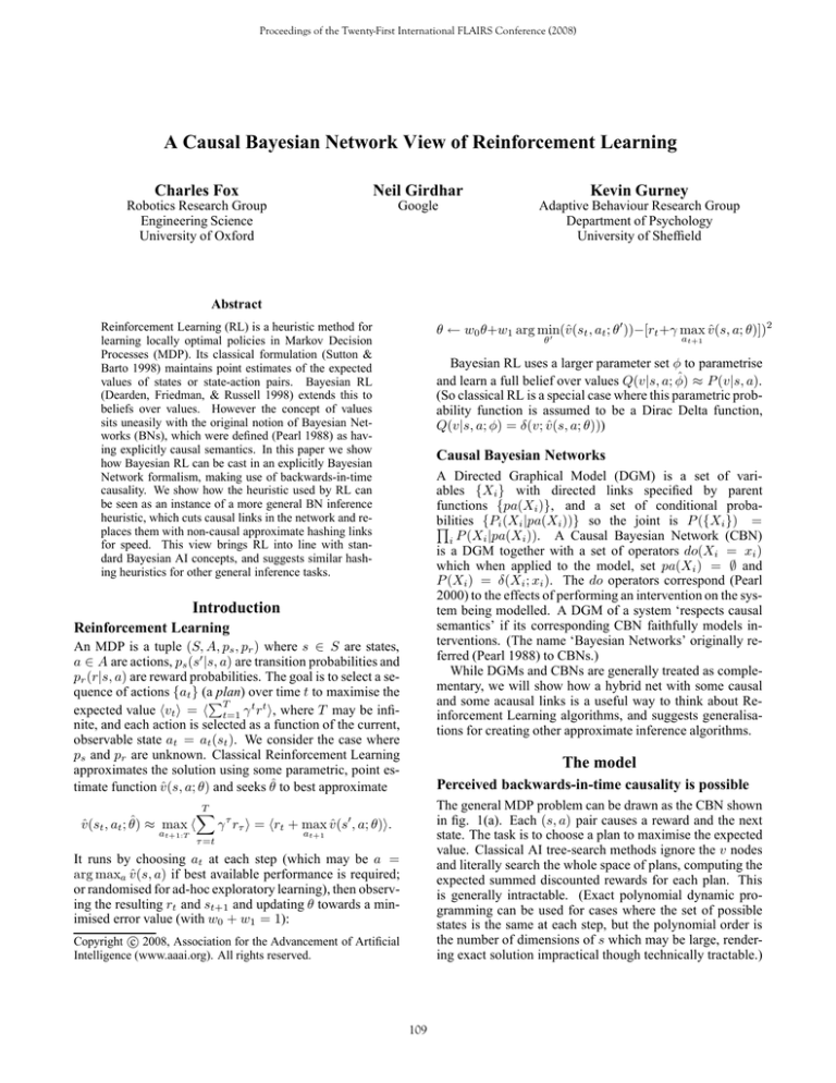
The general MDP problem can be drawn as the CBN shown
in fig. 1(a). Each (s, a) pair causes a reward and the next
state. The task is to choose a plan to maximise the expected
value. Classical AI tree-search methods ignore the v nodes
and literally search the whole space of plans, computing the
expected summed discounted rewards for each plan. This
is generally intractable. (Exact polynomial dynamic programming can be used for cases where the set of possible
states is the same at each step, but the polynomial order is
the number of dimensions of s which may be large, rendering exact solution impractical though technically tractable.)
T
X
v̂(st , at ; θ̂) ≈ max h
γ τ rτ i = hrt + max v̂(s′ , a; θ)i.
at+1:T
τ =t
at+1
θ
at+1
It runs by choosing at at each step (which may be a =
arg maxa v̂(s, a) if best available performance is required;
or randomised for ad-hoc exploratory learning), then observing the resulting rt and st+1 and updating θ towards a minimised error value (with w0 + w1 = 1):
c 2008, Association for the Advancement of Artificial
Copyright Intelligence (www.aaai.org). All rights reserved.
109
v
a1
s1
a1
s2
a2
s3
s2
s1
a2
a3
r1
r2
r3
v1
v2
(a)
v3
s3
a3
s1
a1
time
s2
a2
s3
a3
r1
r2
r3
r1
r2
r3
v1
v2
v3
v1
v2
v3
(b)
In the action selection network shown in fig. 1(b), we
sever all the causal links and replace them with two acausal
links. So we assume an approximate, parametric distribution
Q(vt |st , at ; φ). This is not a causal link: rather it is some
function, whose parameters are to be learned, that will approximate the true causal P (vt |st , at , ât+1 , ...ât+N ) where
aˆi are the actions in the optimal plan given at . It can be
thought of as a ‘hashing’ link, making the best available
guess under limited computational resources.
Once at is thus determined (though not yet executed) the
learning step is performed. We remove the hashing links
and reinstate the two causal links required to exactly update
the parameters of vt , shown in fig. 1(c). We assume that the
best action was selected and will result in vt from the actionselection step (which may be a Delta spike in classical RL or
a belief distribution in Bayesian RL). The previous step’s reward rt−1 is already known, so vt−1 is updated accordingly,
using the standard Classical and Bayesian learning methods
described earlier.
Following the learning step, the results of at are observed
(rt and st+1 ) and the actor phase begins again for t + 1.
(c)
Figure 1: (a) Full inference. (b) RL action. (c) RL learning.
In the unknown ps , pr case they must also infer these probabilities from the results of their actions. Tree-searching
can equivalently be conceived of as using the deterministic vt = γvt+1 + rt nodes to perform the summation. Inference proceeds as before: at each time t, for each plan
(ordered by the classical search algorithm), we instantiate
the plan nodes and infer the distributions over the v nodes,
then perform the first action from the plan with the highest
hvt i. Using message-passing algorithms (Pearl 1988), information must propagate all the way from the left to the right
(via the a nodes) of the network and back again (via the v
and r nodes) to make the inference. This is time-consuming.
The network respects causal semantics, and despite this
it includes arrows pointing backwards through time. This is
not a paradox: the expected discounted reward vt at time t
really is caused by future rewards: that is its meaning and
definition. Note that vt does not measure anything in the
physical world, rather it is a ‘mental construct’. So there is
no backwards causation in the physical world being modelled. But there is backwards causation in the perceptual
world of the decision maker: its percepts of future rewards
cause its percept of the present vt . For example, if vt is
today’s value of a financial derivative, and we are able to
give a delayed-execution instruction now that will somehow
guarantee its value next month, then the causal do semantics
would give a faithful model of this future intervention and an
accurate current value. However value is a ‘construct’ rather
than an object in the physical world, so no physical causality
is violated.
Discussion
Exact inference for action selection in the exact CBN is
time-consuming, requiring inference across the complete
temporal network and back again to evaluate each candidate
in a plan searching algorithm. We have seen how RL can be
viewed as a heuristic which cuts the causal links of the CBN
and replaces them with acausal hashing links, mapping directly from the current state to an approximate solution. We
suggest that having viewed RL in the context of CBNs, a
similar method could be applied to more general inference
problems when cast as CBNs: isolate the time-consuming
parts of the network and replace them with trainable acausal
hashing functions. The process of switching between causal
and hashing links can also be seen in the Helmholtz machine
(Dayan et al. 1995) in a similar spirit to RL.
We also saw how the causal do semantics allow for coherent backwards-in-time causality, where the caused entities
are perceptual ‘constructs’ rather than physical entities. This
makes an interesting contrast to other conceptions of causality such as (Granger 1969) which assume that causality must
act forwards in time.
References
Dayan, P.; Hinton, G. E.; Neal, R.; and Zemel, R. S. 1995.
The Helmholtz machine. Neural Computation.
Dearden, R.; Friedman, N.; and Russell, S. J. 1998.
Bayesian Q-learning. In AAAI/IAAI, 761–768.
Granger, C. W. J. 1969. Investigating causal relations.
Econometrica 37:424–438.
Pearl, J. 1988. Intelligient Reasoning with Probabalistic
Networks. Morgan Kaufmann.
Pearl, J. 2000. Causality. Cambridge University Press.
Sutton, R., and Barto, A. G. 1998. Reinforcement Learning. MIT.
Approximation method
We now present RL as a heuristic method for fast inference
and decision making in the previous CBN. The two steps of
RL, action selection and learning, (also known as the ‘actor’
and ‘critic’ steps) correspond to two DGMs derived from the
CBN. We change the computation of the v nodes, from being
exact to approximate expected discounted rewards. (Their
semantics are the same, they still compute value, but their
computational accuracy changes.)
110