From: Proceedings of the Eleventh International FLAIRS Conference. Copyright © 1998, AAAI (www.aaai.org). All rights reserved.
Propagating
probabilities
in System P
Rachel
Bourne 1 and Simon Parsons
Department of Electronic Engineering.
QueenMasT and ~5,k~stfield Coll(,ge
Univrrsity of London.
London E1 -INS. UK.
Abstract
In this paper we suggest a way of using the rules of
System P to propagate lower bounds on conditional
probabilities. Usinga knowledgebase of default rules
whichart, consideredto be constraints on a probability
distribut ion, the result of applyingthe rules of P gives
us newconstraints that were implicit in the knowledge
base and their associated lower bounds.
Introduction
Default reasoning has been widely studied in artificiM
intelligence,
and a number of formalisms have been
proposed as a means of capturing such reasoning (Ginsberg 1987), most prominent among which are defauh
logic (Reiter 1980) and circumscription (McCarthy
1980). *Iany of these systems, including default logic
and circumscription, have proposed particular merhanisms fi)r defauh, reasoning, and nfight therefore be
considered quite specialised. However, there ha~s also
bee.n work on more general approaches which attempt
to analyse in broader terms what default reasoning
involves. An early attempt to do this was Shoham’s
(1987) proposal that all non-monotonicsystems (’,)uld
be (’.haraeterised in terms of the preference order over
their models. A more proof-theoretic strand of this research has investigated the formal|sat|on of the underlying requirements for any non-monotonic consequence
relation. Perhat)s the most influential piece of work
within this area is that of Kraus et al. (1990).
Kraus et el. investigated tim properties of different sets of Gentzen-style proof rules for non-monet(talc
consequencerelations, and related these sets of rules to
the model-theoretic properties of the associated logics. Their major result was that a particular set of
proof rules had the same model-theoretic properties
that Shoham
had identified for logics in which there is
a preference order over nmdels. This system of proof
rules was termed System P by Kraus et aI., the P
standing for "’preferentiar’.
System P has 1)e,,n the
subject of mu,’h research, and is nowwi,tely ~w(’epted
as the weakest interesting non-moneton|(" system: it.
sanctions the smallest ac(’eptable sot of conclusions
from a set of default statements.
The reason that w[, arc inrer(,strd in the rules of System P is that, in addition to a semantics in terms of a
preference order over mod(,ls, they also haw, n pn)t)ahilistic semami(’s. In parti,’ular, Pearl (1988), following work by Adams (1975), showed that a st,marries
based on infinitesimal prol)abilitios satisfies the rules
of System P. Whih’ the use ,)f infinitesimal prol)abiliti(.s is theoretically interesting, iI b,,’ks s[mwlhingin
practical terms. If we are to use System P to reason at)out the real worhl we will have to write ,h’fmflts
which sunlmm’ise our knowledge about it.. and we may
well be unhappy making statement.s whoso validity depends upon infinitesimal values. To overcomethis difficulty, we suggest using r(’al probabilities Mongwith
the rules of System P, giving each default statt,nmnt a
lower boundedprobability, and showingthat pr,)of:s in
the System P can b(, used t,, propagatr~ t.hose I)ountls
to find out somethingroiwrote about tit(, pr, Jlml)ilily
(ff the derived resuh s.
1Supportedby an EPSRC
studentship.
Copyright
¯ 1998,
American
Association
forkrSficial
Intelligence
(www.aaai.org).
Allrights
resen~l.
440 Bourne
Entailment
in System P
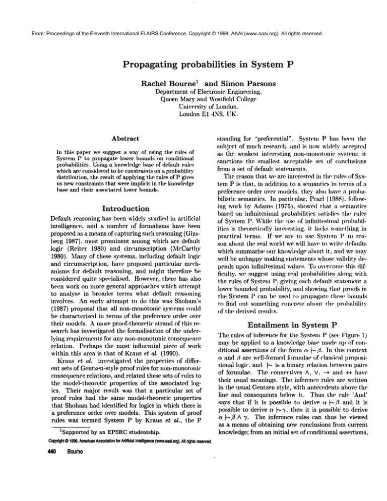
The rules of inference for the System P (see Figure 1)
may be applied to a knowledge base made up of conditional assertions of the form t~ ~--ft. In this context
a and i~ are w(,ll-fiJrmed fi)rmulae of classical prot)ositional logir, and ~, is a binary relation Imtwe(,n pairs
of formulae. The conr,e(’tives A.. V~ -4 and ~-~ have
their usual meanings. The inference rules are written
in the uslrAl Gentzen styh:, with antecedents above the
line and consequents below it.. Thus the rule :And’
says that if it. is possible to derive u ~-,,;’~ and it is
possible to derive ~. ~. ~, then it is possible to derive
a b’,3 A 7- The inference rules can thus he viewed
as a means of obtaining new conclusions from current
knowledge;from an initial set of conditional assertions,
a ~ a
Reflexivity
ab’ ’
,’3
a ~,,’~"
Left Logical Equivalence
Right Weakening
And
Cmltious Monotonicity
Figure 1: Rules of System P
further conditional assertions may be obtained by applying the rules.
Twothings should be noted about the set of rules in
Figure 1. Firstly, they only tell us howto derive new
conditional assertions. If we wish to kmowwhether we
are justified in inferring a new fact, say" %given that
we currently know some other fact, say a, and this
is all we know. it is necessary to deternfine whether
o ~,, "~ is derivable from our knowledgebase of conditional assertions. Secondly, the proof rules in Figure 1
form a minimal set sufficient to characterise System P.
Other rules may be derived from them in mudl the
same way that new conditional assertions are derived.
Twosuch rules are given in Figure 2; Cut which allows the elimination of a conjunct from the antecedent
side, and S which allows the derivation of a material
implication. Both of these (as we shall see later in the
paper) may be derived directly by the application of
the basic rules.
The semantics for System P introduced by Adams
makes the assumption that the propositional variables
are the basis of an unspecified joint probability distribution which is constrained by the conditional assertions. These conditionals are taken to tel)resent conditional probabilities of the consequent given the antecedent being greater than or equal to 1 - e for any
e > 0, that is:
a ~ 3 represents
P(3la) > - e for al l e > O.(1)
Probabilistic consistency is defined as the existence
of at least one probability, distribution which satisfies
these constraints (Adams1975); probabilistic entailment. of a further conditional is defined as probabilistic
aA3 I~7
a F3~
Cut
S
Figure 2: Twoderived rules of System P
inconsistency of its counterpart, that is:
a ~ 3 is p-entailed by A iff A U {a [-,--B} is pinconsistent,
This implies that all probability distributions that satisfy A also satis~, o ~ B. Howeverthis result mayonly
be acahieved by using infinitesimal analysis so that the
derived conditional will be constrained to be greater
than 1 - 5 for any 5 :> 0 if the e of the original conditionals is made small enough. This can be paraphrased
as saying that System P aUowsus to make our conclusions as (’lose to certainty as we like, provided the conditional probabilities associated with the conditional
assertions are sufficiently close to certainty. In the literature this is used to justify the conclusions drawnby
using SystemP; ff we are sure of the (xmditional assert.ions and so are willing to give them high conditional
probabilities, then the conditional assertions derived
from them will ’also have high probabilities.
However,using this interpretation of the rules means
assuming that we ate able t,o give the conditional assertions arbitrarily high conditional probabilities. This
is fine in the case that the assertions are pie(’es of default knowledge which are felt to hokl almost all of
the time. However,with less reliable information, for
which e is not infinitesimal, it s(~ms less justifiable to
accept the infinitesimal mmlysis. In particular, if a set
of conditional assertions are used to derive newa.ssertions ~mdthese new assertions are themsch’es used as
the basis for new dedu(’tions, then it seems likely that
somee values will be far from infinitesimal. Becauseof
this concern, this paper investigates the impact of noninfinitesimal e values by considering what happens to
values of ~ and ~ whenthe rules of P are applied. The
result is twofold. First it is possibh: to track the effect of non-infinitesimal values, and second it becomes
possible to identify- bounds on the actual conditional
probability of derived assertions.
Usingreal e-values
Weassociate with each conditional assertion au e-value
which represents, for o’ ~,, 3, an upper bound on the
conditional probability P(-~BIa). Wedemonstrate how
using these values for each original conditional, we cazl
Uncertainty
Reasoning
4141
0
0
P(o)(1P(fl)(1 -max{0, P(a) + P([3) 1}
¯ max{0,P(a’ A 7) + P(,3 A"r) --
<
<
_<
_<
_<
_<
P(a)
P(i3)
P(a A "))
< 1
< 1
< P(o)
P(.3^ ~.)
<_ P(/3)
P(a A fl)
P(a Ai] A "))
<_ min{P(a)..P(fl)}
<, min{P(caA7),P(flAq’),P(oAiJ)}
Figure 3: The constraints for ()r.
generate ti vahles for the output conclusions. This enables us to calculate the lower boundon tile I)robability
of a conclusion based on the proof steps used to derive
it. Weconsider first tile six basic rules of System P,
and then use the results obtained for those rules to
obt,~fin results for S and Cut.
Reflexivity: A reflexive conditional assertion m~, be
introduced at any stage in a proof, and, since P(alo)
1 for all formulae a. any such conditional will have ml
c-value of zero.
Left Logical Equivalence: This rule me.ans that
we may take any conditional assertion and replace
its antecedent with a logically equivalent expression.
Clearly, the derived conditional will have the same evalue as the original one.
Right Weakening: Right Weakening involv(,s
relfiacing the COlmetluent of a conditional with any expression classically derivable from it. Now,::1 -4 ~.
meansthe models of fl are a subset of the models of ~,
,’md hence:
P(q. a) >_P(fl.
Weare required to nfiifimize this expression subject to
lhe constraints:
1 - ~i <_
<_ 1
P(i3]t~)
1- e2 _<
P(q[a)
<_ 1
0 _< P(q;la’.-~fl) g 1
Equation (4) is linear in P(7]a) and P(?,:I a, ~:3) and
will therefore attain its ininimumwhenP(a.I a) is nfininmmand P(?’I o, W3)is maximum.This givt;s us:
P(.’3la))
e(i3la)
(I - el) - (1 -
P(~Ir~,;3)>__
> 1.
P(/~la)
which will I)e ufinimum when P(/3l~t) is mininumL
This gives us all ~-value for the derived rule n A,’.3 ~ ~,,
of:
~-’2
I --~l
And: This time we are interested
sider:
in P(fl, ~1o). Colt-
P(a,/3. "~)
Now,since:
l’(n)
i,(~.la) P(%P(a----~’
(~)
P(,,’3,
(~)
P(i3I,~)P(c~)
P(a, :3, ~,’)P(o,
P(a, ,,3)P(a)
= P(’da,,3)P(i3lu)
it follows that:
P(?la) > P(/3la)
(’2)
and therefore the c-value of a rule obtained by Right
Weakeningwill not be h’u’ger than the ,-vMue of tile
rule fi’om which it was obtained. Since we are dealing
with lower bounds, we mayuse the stone value for the
derived rule.
Cautious Monotonicity: Here w(’ are interested
the value of P(’)’]t~’. fl). Now:
in
P(n’la) = P(z, la, ’3)P(flla) P(Tla, ~’3)P(~/~la) (3
Substituting 1 - P(Bla) for P("~Bla) and reaxranging,
we obtain
P(?la, ~) :- P(91a)- (1 - P(.810))P(~,la,-~,3) (4)
P(flla)
442 Bourne
(5)
We,are required to minimizethis expression subject to
the constrmnts:
1-el _< 1’(.’31o)
_(
1 - e2 < P(TIo) < 1
and in the previous case we saw that these constraints
ilnply that:
1 - e----Z---2 < P(’~’la, 3) <_ 1
1 -¢1 Equation (5) will be minimumwhen both factors
the product on file right-hand side are, so that
(6)
Reflexivity
Left Logical Equivalence
Right Weakening
And
Cautious Monotonicity
a ~"~1 7, .3 ~2 7
Or
Cut
Figure 4: Rules with associated bounds
which, as wewouldexpect, is symmetricalin el and e2.
This gives us an e-value for the derivedrule of ~l + e2.
Or: For this rule we want to know the value of
P(7[a V .q). This is slightly moretricky than previous cases since the necessaryequation cannot be solved
analytically. However
there is a flmction whichapproximates the lower houndclosely for small ovahmsarid is
no worsethan 10%lower th,’m it even for large values.
Considertile following:
P(’,le~ v 3)
P(e~ A 7) + P(fl A 7) - P(~*A 3 A
P(o) P(fl) - P(a A
Weare required to minimizethis expression subject to
the constraints of Figure 3. This is a non-linear optimisation problem whidl we can easily solve numerically over the specified range. A simple brute force
search shows that the function is boundedbeh)w by
(1 - et )(1 - e2) whichgives us an e-value for the
rivedrule of e~+ e,_, - e~e,,.
For completeness sake. we exmninethe derived rules
Cut and S since they are the most usefifl rules when
proving things. Ib makethe presentation clearer we
have denotedby ~--,, a conditionMwith e-value of el.
S: For S weneedto deriw~c~ ~ ...... fl --~ 7 and the
value of e,,,,,,, fromn Afl ~,, 7 just using the basic
rules. This earl be done as follows. First apply Right
Weakening
to a’ Afl b’~, ~, to get:
a A3N~,7,1= 7 ~ (3 -~ 7)
0")
Wethen apply Reflexivity followed by Right Weakening (twice) to a A -’3 to get:
c~A-~S
b~o~A-~;~,I=~,,’~-~(;~--~7)
a A-~3No/J-+’,
(8)
Then we combine(7) and (8) using Or and apply
Logical Equivalenceto get:
orA~ N,,fl -~ 7,a A"-1,’3~’,,0.’3 --~ "7
a N~,3-~7
Theconsequentof this last derivation is the consequent
of S: and comparingthis with the antecedent, we can
see that applying S has no effect on tile e-value; the
value for the derived conditional assertion is the same
as for the original assertion.
Cut: For Cut, weneed to discover howa ~ ....... "~"
maybe derived from c~ A fl ~ 7 and t~ ~ i~. This
turns out to be easy given the result for S. S tells us
that the e-value of a N 3 -+ ~ is the same as that
of a A fl b" 7, so we have a N,~ fl -~ ? and applying
Andto a N¢~fl ~ ~,. and a N,o ’3, followed by Right
Weakeninggives:
Cut is thus proved, and the e-value for its conseq~mnt
established.
In obtaining these results, wchaveshownthat using
each of the rules of P, and henceany derived rules, we
can obtain lower boundson the conditional probability
of tile conchmiongiven those of the antecedents. Figure 4 showstile basic rules plus S and Cut annotated
with lower probability boundson antecedents and consequents. It is clear that these lower boundsnever
improve. Using rules Andand Or, or rules derived
from these, meansadding the e-values so that. after
only a few proof steps our conclusionsmayattain high
e-values. A high ~-value meansthat the lower boundon
the associatedconditional probability is lowand if this
becomestoo low then we don’t have muchinformation
about the probability since the upper boundis always
1. Clearly, therefore, our input values must either be
Uncertainty
Reasoning
443
(i)
linda A steve }"o.os -~noisy, linda ~"o., steve
linda ~"o.15 -~noisy
Cut 4.5
(ii)
linda }"o.15-moisy, linda ~"o.oa great
li.nda ~o.,6 great A -~noisy
And (i),2
(iii) T ~"o.ls --,linda V (great A -mtoisy), T ~’-o., noisy V -,great
T ~"o.’.,e, ~linda
(i)
lin.da ~o.a steve, linda ~o.ot .qreat
linda A steve ~o.ol l great
(ii)
linda A steve ~o.o~-m~.oisy, linda A stc.vc ~’~0,(}1
li’nda A steve ~o.o6, great A -~.noisy
S. And(ii),7.
R~N
C.M.1.2
I
great
And5.(i)
Figure 5: Proofs of 7- I,~0.._,s -,linda and linda A stcvc ~o.ou1great A -,noisy
extremely small or our proofs short in order to obtain
uscfifl results. However. as our example shows, these
conditions can be met without too much imagination.
Example
The following was inspired by examples given by Kraus
et al. (Kraus, Lehmann, & .Magidor 1990).
Brian and Linda are two happy-go-hwky people
whoare normally the life and soul of any party (so
if either go to a party it will normally be great).
Until recently Brian and Linda were married, but
then Linda ran off with a nfime artist, Steve. As
a re.suit, if both Brian and Linda go to the same
party they will l)robably have a screaming row and
ruin it (so it will not be great, anti it will be noisy).
If Linda goes to a party she will probably take her
new boyfriend Steve and get him to entertain the
guests with his marvellous miming. Thus if Linda
goes to a party, Steve will probably go to the santo
party and if Linda and Steve go to a party together
it will normally not be noisy because everyone will
be watching his minting. Normally parties that
great are noisy and those that are not noisy are
not great.
Werepresent this by the following rules and e-vahms:
It should he understood that we are trying to ascertain the likelihood of any given party having various
attributes (brian is present, it is noisy, and so on).
1.
2.
3.
4.
brian ~o.o~ great
linda b’o.ol great
brian A linda ~o.15 -,great A noisy
linda ~o.1 steve
444 Boume
5. lin.da A stevc t"..o,~ --moisy
6. great ~"o.l noisy
7. ~noisy ~o.I -~9rt at
Figure 5 gives proofs fi~r two new conditionals with justifications on the right and e-values propagated ahmg
the way. T denotes arty tautology. The first of these
given us the lower bound on the l)mtmbility of Linda.
not a! tending maypart icular party given what woknow
(which is what the T on the anteced(,nt side nmans).
Rememberingthe denotation of (1), T ~u.’_,t;-,linda
nleans
that:
l’(~lindalT)
P(-~linda!T)
k l- 0.26
> 0.7.1
fi’om which we cml conclude that Lin,la is unlikely to
go to any particular party. However.this doos not stop
us drawing conclusions al)out parti~.s which we know
/.hat, Linda does go to. indeed, Figure 5 showsslt(’h
conclusion:
linda A steve ~0.061 .qrcot A -.noisy
meansthat if Linda and Stove go to a l)arty., then the
probability that it. is both great mid -~.aaisy is greater
than 0.94. These results show that using our nmthod
we can obtain usable numerical results from an initial
set of defaults.
This is particularly useflfl in unexpectedor unlikely
circumstances (as in the case that we knowLinda goes
to a party) since such cases could not be captured in
classical logic. To see this point consider what. would
happen if we translated part of our knowledge about
parties into propositional logic:
1.
2.
3.
4.
linda
great
linda
linda
D great
D noisy
D steve
A steve D -~noisy
From the first two sentences we could conclude noisy,
from the first, third and fourth sentences we could conelude -~noisy and with the two we would have an inconsistency. What System P does is to balance the
effects that Linda and Steve have on a party and our
approach extends this to allow us to predict just how
likely the balanced outcome is.
Conclusion
Wehave slmwn that given the assumption that comtitional assertions m~, be treated as conditional probabilities with lower bounds, we can obtain lower bounds
for the derived conclusions. Thus if we knowthe lower
bounds on the conditional probabilities of a set of input assertions, we can establish the lower bounds on
the conditional probabilities of the derived assertions.
Moreover these are given by simple functions of the
initial bounds calculated for each proof step in System
P. One advantage of this approach is that it "allows us
to use real rather than infinitesimal probabilities since
by keeping track of the bounds we can tell which conclusions are justified;clearly any conclusion with a low
lower bound might be considered suspect. Another
advantage of this method is that only a lower bound
conditional probability is required for each default rule
rather than a point probability,
and this may mean
that the numerical values are easier to assess. Clearly
wc still require these values to be high or the results
obtained will be useless since derived conditionals will
only be knownto have an associated conditional probability that is greater than somesmall value.
There are two drawbacks to this approach which
should be mentioned. Firstly System P is accepted
as being a sceptical reasoning mechanism,that is, only
conservative (and completely sound) conclusions can
be obtained. This is insufficient
for most purposes
since we will often want to draw more tenuous conclusions. However,specialisations have been suggested
(Goldszmidt, Morris, & Pearl 1993; Pearl 1990) aud
maybe possible for our approach to be extended in this
direction. Secondly, despite the appearance of the rules
of System P, it is not knownwhether a feasible procedure for proof generation exists; a model-theoretic procedure for determining p-entailment (which guarantees
a proof) exists but the complexity prevents realistic
applications.
Naturally for our approach to be acceptable, it is
necessary to accept that defaults may be reasonably
taken to be statements about probabilities, in particular constraints on a joint probability distribution which
describes the state of the world. While this is natural
from a Bayesian perspective, it might seem more questionable to some. However, we feel that the position
can be justified from a pragmatic perspective as well.
Using probability to say what. defaults meangives them
a semantics which is comparatively simple, at least at
an informal level, and one which could, with our extension, be used in conjunction with real data about the
world. This seems a good justification
for accepting
the semantics, in our opinion it is clearer and therefore
more plausible than other default reasoning systems.
Any reasoning nmchanismthat is required to treat defaults in a uniform way must have some representation
for them. Humansmay use default rules in different
waysin differing conte~xts., but if we wish to buiht practical reasoning systems, we must find systematic ways
to approximate defaults. If this leads to making some
assumptions then, so long as they are clear, so be it.
Wewill achieve nothing unless we have a firm basis for
saying what we mean by a default.
References
Adams, E. 1975. The Logic o/ Conditionals.
drecht, Netherlands: Reidel.
Dor-
Ginsberg, M. L., ed. 1987. Readings in Nonmonotonic
Reasoning. San Mateo, CA: Morgan Kaufmvam.
Goldszmidt, M.; Morris, P.; mad Pearl, J. 1993. A
maxiInum entropy approach to nonnmnotonic reasoning. IEEE Transactions on Pattern Analysis and Machine Intelligence 15:220 232.
Kraus, S.; Lehmann, D.; and Magidor: M. 1990. Nonmonotonic reasoning, preferential models and cunmlative logics. Artificial Intelligence 44:167--207.
McCarthy, J. 1980. Circumscription---a form of nonmonotonicreasoning. Artificial Intelligence 13:27--39.
Pearl, J. 1988. Probabilistic Reasoningin Intelligent
Systems: Networksof Plausible Infe~v, nce. San Mateo,
CA: Morgan Kaufmann.
Pearl, J. 1990. System Z: a natural ordering of defaults with tractable applications to defanlt reasoning. In Proceedings of the 3rd Conference on Theoretical Aspects of Reasoning about Knowledge, 121-135.
l~iter, R. 1980. A logic for default reasoning. Artificial Intelligence 13:81-132.
Shohmn: Y. 1987. Nonmonotonic logics: meaning
and utility. In Proceedings of the lOth International
Joint Conference on Artificial Intelligence, 388 393.
UncertaintyReasoning
445