An enhanced representation of time series which allows fast and accurate
classification,
clustering and relevance feedback
From: AAAI Technical Report WS-98-07. Compilation copyright © 1998, AAAI (www.aaai.org). All rights reserved.
EamonnJ. Keoghand Michael J. Pazzani
Departmentof Informationand ComputerScience
Universityof California, Irvine, California 92697USA
{ pazzani,eamonn
} @its .uci.edu
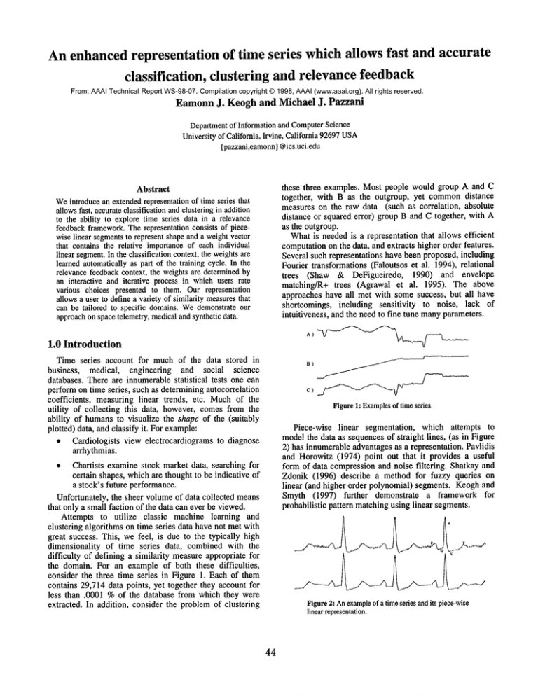
these three examples. Most people would group A and C
together, with B as the outgroup, yet commondistance
measures on the raw data (such as correlation, absolute
distance or squared error) group B and C together, with
as the outgroup.
Whatis needed is a representation that allows efficient
computationon the data, and extracts higher order features.
Several such representations have been proposed, including
Fourier transformations (Faloutsos et al. 1994), relational
trees (Shaw & DeFigueiredo,
1990) and envelope
matching/R+ trees (Agrawal et al. 1995). The above
approaches have all met with somesuccess, but all have
shortcomings, including sensitivity to noise, lack of
intuitiveness, and the need to fine tune manyparameters.
Abstract
Weintroducean extendedrepresentationof time series that
allowsfast, accurateclassificationandclusteringin addition
to the ability to explore time series data in a relevance
feedbackframework.Therepresentation consists of piecewiselinear segmentsto represent shapeand a weightvector
that contains the relative importanceof each individual
linear segment.In the classification context,the weightsare
learnedautomaticallyas part of the training cycle. In the
relevancefeedbackcontext, the weightsare determinedby
an interactive and iterative process in whichusers rate
various choices presented to them. Our representation
allowsa user to define a variety of similarity measuresthat
can be tailored to specific domains.Wedemonstrateour
approachon spacetelemetry,medicaland syntheticdata.
1.0 Introduction
:
Time series account for much of the data stored in
business, medical, engineering and social science
databases. There are innumerablestatistical tests one can
perform on time series, such as determining autocorrelation
coefficients, measuring linear trends, etc. Muchof the
utility of collecting this data, however, comes from the
ability of humansto visualize the shape of the (suitably
plotted) data, and classify it. For example:
* Cardiologists view electrocardiograms to diagnose
arrhythmias.
Figure
1: Examples
of timeseries.
¯
Chartists examinestock market data, searching for
certain shapes, which are thought to be indicative of
a stock’s future performance.
Unfortunately, the sheer volumeof data collected means
that only a small faction of the data can ever be viewed.
Attempts to utilize classic machine learning and
clustering algorithms on time series data have not met with
great success. This, we feel, is due to the typically high
dimensionality of time series data, combined with the
difficulty of defining a similarity measureappropriate for
the domain. For an example of both these difficulties,
consider the three time series in Figure 1. Each of them
contains 29,714 data points, yet together they account for
less than .0001%of the database from which they were
extracted. In addition, consider the problemof clustering
44
Piece-wise linear segmentation, which attempts to
modelthe data as sequencesof straight lines, (as in Figure
2) has innumerableadvantages as a representation. Pavlidis
and Horowitz (1974) point out that it provides a useful
form of data compression and noise filtering. Shatkay and
Zdonik (1996) describe a method for fuzzy queries
linear (and higher order polynomial) segments. Keoghand
Smyth (1997) further demonstrate a framework for
probabilistic pattern matchingusing linear segments.
Figure
2: Anexample
of a timeseriesandits piece-wise
linearrepresentation.
Although pattern matching using piece-wise linear
segments has met with somesuccess, we believe it has a
major shortcoming. Whencomparingtwo time series to see
if they are similar, all segments are considered to have
equal importance. In practice, however, one maywish to
assign different levels of importanceto different parts of
the time series. As an example, consider the problem of
pattern matchingwith electrocardiograms. If a cardiologist
is attempting tO diagnose a recent myocardial infarction
(MI) she will pay close attention to the S-T wave, and
downplay the importance
of the rest of the
electrocardiogram. If we wish an algorithm to reproduce
the cardiologist’s ability, we need a representation that
allows us to weight different parts of a time series
differently.
In this paper, we propose such a representation. Weuse
piece-wise linear segmentsto represent the shape of a time
series, and a weight vector that contains the relative
importance of each individual linear segment. Wewill
show that this representation allows fast and accurate
clustering and classification. Additionally, we will show
that this representation allows us to apply relevance
feedback techniques from the information retrieval
literature to time series databases.
The rest of this paper is organized as follows. Section 2
introduces notation and two important operators. Section 3
demonstrates howthese techniques are used for relevance
feedback, and section 4 describes a classification algorithm
which takes advantage of our representation to greatly
boost accuracy.
.
(AxRi,AYai)
f(t)
I
I
r~
t
i~ ::Aw
Figure
3: Werepresenttimesseriesbya sequence
of straight
segments,
togetherwitha sequence
of weights(shown
as the
histogram)
whichcontainthe relativeimportance
of eachsegment.
After a time series is segmentedto obtain a sequence, we
initialize all the weights to one. Thereafter, if any of the
weights are changed, the weights are renormalized such
that the sumof the products of each weight with the length
of its corresponding segment, equals the length of the
entire sequence, so that the following is alwaystrue:
K
W i * ( AXRi- AXLi) = AXRk- AXLI
~--,i=l
This renormalization is important because it gives the
following property: the total weight associated with a
sequence of a given length is constant, regardless of how
manysegments are used to represent it. Therefore, any
operation that changes a weight has the effect of
redistributing all the weights. For example,if the weightof
a single segmentis decreased, all other segmentswill have
their weight slightly increased. So the weights reflect the
relative, not absolute, importanceof the segments.
2.0 Representationof time series
There are numerousalgorithms available for segmenting
time series, manyof which where pioneered by Pavlidis
and Horowitz (1974). An open question is how to best
choose K, the ’optimal’ number of segments used to
represent a particular time series. This probleminvolves a
trade-off between accuracy and compactness, and clearly
has no general solution. For this paper, we utilize the
segmentation algorithm proposed in Keogh (1997). This
methodsegments a time series, and automatically selects
the best value for K. Weemphasize, however, that all the
algorithms presented in this paper will work regardless of
howthe segmentation has obtained.
2.2 Comparingtime series
An advantage in using the piece-wise linear segment
representation is that it allows one to define a variety of
distance measures to represent the distance between two
time series. This is important, because in various domains,
different properties maybe required of a distance measure.
Figure 4 shows some of the various distortions one can
encounter in time series, and we briefly consider each
below.
The segmentation algorithm, which produces the
sequences, acts as a noise filter, so we do not need to
consider handling noise directly (Pavlidis and Horowitz
1974, Keogh 1997). Most domains require a distance
measure that is insensitive to offset translation. As an
example, consider two stocks, whose values fluctuate
around $100 and $20 respectively. It is possible that the
stock movementsare very similar, but are separated by a
constant amount.
Amplitudescaling, where two sequences are alike, but
one has been ’stretched’ or ’compressed’in the y-axis, can
be dealt with easily. It simply requires normalizing the
sequences before applying the distance operator. Agrawal
et al. (1995) describe howto do this with raw time series.
Normalizing with sequences is similar, but can be
accomplished klK times faster. Dealing with longitudinal
2.1 Notation
For clarity we will refer to ’raw’, unprocessedtemporal
data as time series, and a piece-wise representation of a
time series as a sequence. Wewill use the following
notation throughout this paper. A time series, sampledat k
points, is represented as an uppercaseletter such as A. The
segmentedversion of A, containing K linear segments, is
denoted as a bold uppercase letter such as A, where A is a
5-tuple of vectors of length K.
A - { AXL,AXR,AYL,AYR,AW}
The i ~ segment of sequence A is represented by the line
between (AXL1 AYLi) and (AXR~AYR,), and Aw~, which
represents the segments weight. Figure 3 illustrates this
notation.
45
the experiments in this paper we used the simple distance
measure given below. This measure is designed to be
insensitive to offset translation,
linear trends and
discontinuities.
It is convenient for notational purposes to assume that
the endpoints of the two sequences being compared are
aligned, as in Figure 5. In general, with real data, this is not
the case. So we will have to process the sequences first, by
breaking somesegments at a point which corresponds to an
endpoint in the other sequence. This can be done in O(K).
scaling (’stretching’ or ’compressing’in the time-axis)
possible, but muchmoredifficult. Werefer the interested
reader to Keogh1997.
Offset
Translation
~%W
Aznplitude
Scaling
~s
Longitudinal
caling
/~
r, Aw~* Bw~* I( AYL - BYL )-( AYR -BYRi)I
D(A,B)=~
i
i
i
Intuitively,
this metric measures how close
corresponding segments from A and B are to being
parallel. Notethat it has the followingdesirable properties:
Linear
Drift
~
Discontinuities
Figure
4" Some
of the difficultiesencountered
in defininga distance
measure
for timeseries.
Linear drift occurs naturally in manydomains. As an
example, consider two time series, which measure the
absolute sales of ice cream in two cities with similar
climates and populations. Wewould expect the two time
series to be very similar, but if one city’s population
remains constant while the other experiences steady
growth, we will see linear drift. It is possible to remove
linear trends (Box and Jenkins 1970), but it
computationally expensive. However,using the segmented
representation, it is possible to define a distance measure
that is insensitive to linear drift (see below).
Finally, manydatasets (including the Shuttle dataset
referred to in section 4.2) contain discontinuities. Theseare
typically sensor calibration artifacts, but mayhave other
causes. Again, one could attempt to find and removethem,
but our approach is to simply define a distance measure
that is (relatively) insensitive to them
It is possible to define distance measuresfor sequences
that are invariant to any subset of the abovedistortions. For
By’
D(A,B)= D(B,A)
D(A,B)> 0
D(A,A)=
D(A,B) =
--->
A= B
Another important property is that it is efficient to
compute. In particular, comparing two sequences A and B
is approximately k/K faster than comparing the two
corresponding time series A and B. This is especially
important as one mayneed to calculate distance frequently.
For example, supposeone wishes to hierarchically cluster n
data items using a group average method. This requires
O(n3) comparisons. The time series represented by the
sequences shownin Figure 6 contain 29,714 data points,
but their sequence representations contain only an average
of 35 segments. This results in a speedupof 29,714 / 35
848.
\
BYRi
f(t)
I
AvLi
AYRi
I
AXLi
i
b.
t
Figure
6" Anexample
of hierarchically
clusteredtimeseries.
AXR
2.3 Mergingtime series
In this section we define an operation on sequences
which we call ’merge’. The merge operator allows us to
combine information from two sequences, and repeated
Figure5: Comparing
twotimeseries is equivalentto summing
the
absolutedifference
between
the pair of dashlines, (weighted
by
the appropriate
weighting
factor)for everysegment.
46
application of the merge operator allows us to combine
information from multiple sequences. The basic idea is that
the merge operator takes two sequences as input, and
returns a single sequence whose shape is a compromise
between the two original sequences, and whose weight
vector reflects how muchcorresponding segments in each
sequence agree. As in the distance operator we assumethat
the endpoints of the sequenceare aligned.
Whenmerging sequences one may wish for one of the
two input sequences to contribute more to the final
sequence than the other does. To accommodatethis, we
associate a term called ’influence’ with each of the input
sequences. The influence term associated with a sequence
S is a scalar, denoted as SI, and may be informally
considered a ’mixing weight’. Wherethe influence term
comesfrom depends on the application and is discussed in
detail in sections 3.1 and 4.1 below.
To merge the two sequences A and B with influence
terms AI and BI respectively,
we use the following
algorithm that creates the sequence C:
if (AI * BI < O) then
else
end
A
B
_/\
----/
....._
/ X ____._____.__--.-
ll)
1) C =merge([A,1],[B,
2)
C= merge([A,0.2l,[B,l])
3)
C=merge([A,1],[B,-0.4])
Figure 7:Examplesof the mergeoperator with various influence terms.
1) With two equal influence terms, the shape of the resultant sequence
C is "halfway" between A and B,
WithB’s influence term muchlarger than A’s, the shape of the
2)
resulting sequence C is muchcloser to B than A.
Witha negative influence term for B the shape of the resulting
3)
sequence C looks like A where the differences between A and B
have been exaggerated.
sign = -i
sign = 1
mag = min(IAI[, [BII) / max(lAI[, IBI[)
scale = max(max(AeL), (AYR))
min(min
(Ayr,), (AYR))
for i = 1 to K
CXLi =
i AxL
CXRi i
= AXR
CYLi = ( (AYLi * AI)+(BYL
i * BI)) /(AI+BI)
CYRi = ( (AYRi * AI)+(BYR
i * BI)) / (AI+BI)
run
= AXRi Axl
i
rise = I(AYLi- BYLI)-(AYRi- BYRi) [
diff = (rise / run) * scale
Cwi = (Awi*Bwi) * (l+ (sign * mag)/ (i
diff)
end
Cw = normalize(Cw)
following manner. Wehave a model sequence A, which is
a typical example of a class of sequences. If we merge
sequence A with sequence B, another memberof the same
class, the resultant sequence C can be considered a more
general modelfor the class. In particular the differences in
shape are minimized by averaging, and the weights for
similar segmentsare increased.
In contrast, creating a prototype from both positive and
negative examples uses a negative influence for the
negative examples. As before, suppose we have a sequence
A, which is an example of one class of sequences.
However,suppose B is an exampleof a different class. If
we mergeA with B, using a negative influence term for B,
the resultant sequence C is a newprototype for A’s class
where the differences in shape between A and B are
exaggerated and the weights for similar segments are
decreased.
The above maps neatly to our intuitions. If we are
learning a prototype for a class of sequences from a set of
positive examples, we want the shape learned to be an
average of all the examples, and we want to increase the
weight of segments that are similar, because those
segments are good predictors of the class. If however, we
are trying to learn from a negative example, we want to
exaggerate the differences in shape between classes, and
decrease the weight of similar segments, because segments
that are similar across classes have no discriminatory
power.
Figure 7.3 shows an illustration
of learning from a
negative example. The negative example is given a
Table I: The mergealgorithm.
Figure 7 shows two sequences that have been merged
with various values for the influence terms. Note that the
resultant sequence is more like the sequence with the
higher influence. Note also that the weights are more
differentiated the closer the two influence terms are to each
other. This is because neither sequence is dominating, and
the maximumamount of compromise is taking place. As
you would expect, the trivial
operations
C =
merge([A,AI],[B,0]) and C = merge([A,AI],[A,AI])
result in C = A.
2.4 Learning prototypes
Although the merge operator is designed to be a
componentin the more sophisticated algorithms presented
below, it can, by itself, be considered a simple learning
algorithm that creates a prototypical sequence. Creating a
prototype solely from positive examples works in the
47
negative influence term. As before the magnitude of the
influence term reflects how much the corresponding
sequenceaffects the resultant sequence.
3)
Sin(x
Tan(Sin(xS))
3.0 Relevancefeedback
Relevance feedback is the reformulation of a search
query in response to feedback provided by the user for the
results of previous versions of the query. It has an
extensive history in the text domain, dating back to
Rocchio’s classic paper (1971). Recently, there have been
attempts to utilize relevance feedback techniques in other
domains, notably the MARS
project (Rui et al. 1997).
However,to the best of the authors’ knowledge,no one has
attempted explore time series databases in a relevance
feedback framework, in spite of the fact that relevance
feedback has been shown to significantly improve the
querying process in text databases (Salton &Buckley, 90).
In this section we present a simple relevance feedback
algorithm which utilizes our representation
and we
demonstrateit on a synthetic dataset.
c)
Figure8: Syntheticdatacreatedfor relevance
feedback
experiment.
A) Theoriginaltimeseries.
B) Theoriginaltimeserieswithnoiseadded.
versionof the timeseries.
C) Thesegmented
Our relevance feedback algorithm works in the
following manner. An initial query sequence Q is used to
rank all sequences in the database (this query maybe hand
drawn by the user). Only the best n sequences are shown
to the user. The user assigns influences to each of n
sequences. A positive influence is given to sequences that
the user approves of. Negative influences are given to
sequencesthat the user finds irrelevant.
The relative magnitude of influence terms reflects how
strongly the user feels about the sequences. So if a user
"likes" Si twice as muchas Sj he can assign influences of
1,V2or 2,1 etc. The sequences are then mergedto producea
new query, and the process can be repeated as often as
desired.
Q..~
= merge(
[Q....
Qo~J],
[%,S~I],
[S~,S~I]
.....
[S.,SJ]
)
I
O..w= Qo~al+ s~I+ S21+ ..÷ S.I
3.1 Experimentalresults
To test the above algorithm, we conducted the following
experiment. Weconstructed 500 "Type A", and 500 "Type
B" time series, whichare defined as follows:
¯
¯
Type A." Sin(x s) normalized to be between zero and
one, plus Gaussiannoise with ff =. 1
-2 < x < 2
Type B: Tan(Sin(xS)) normalized to be between
and one, plus Gaussian noise with o = .1 -2 < x < 2
The time series, which were originally sampled at 800
points, were segmented. Figure 8 shows an example of
each type. Note that they are superficially very similar,
although Type B has a somewhatsharper peak and valley.
Webuilt an initial query by averaging all 1,000 time series
and segmentingthe result.
Twenty-five experimental runs where made. Each run
consisted of the following steps. A coin toss decided
whether Type A or Type B was to be the "target" shape
48
(that is, the shape to be considered "relevant" for that
particular experiential run). The initial query was made,
and the quality of the ranked sequences was measured as
defined below. The best 15 sequences were shown to the
user, who then rated them by assigning influences that
reflected howclosely he thought they resembled the target
shape. A new query was built and the search/rate process
was repeated twice more.
We evaluated the effectiveness of the approach by
measuring the average precision of the top 15 sequences,
and the precision at the 25, 50 and 75 percent recall points.
Precision (P) is defined as the proportion of the returned
sequences which are deemedrelevant, and recall (R)
defined as the proportion of relevant items which are
retrieved from the database. These results are shownin
Table 2.
In order to see if the ability to assign negative influence
terms is helpful, we did the following. For each
experimental run we also built queries whichcontained just
the feedback from the sequences judged relevant. These
results are shownin parentheses in Table 2.
Initial QuerySecond Quer7 ThirdQuer,/
P of top 15
.51
.91(.68)
.97t.72)
P~%R
.52
.91(,69}
.96~.71)
P at 50%R
.49
.89<.66)
.95t.69)
P at 75%R
.51
.87(.63)
.95{.68)
Table2: Resultsof relevancefeedback
experiments.
Thevalues
recorded
in parentheses
arefor thequeriesbuilt just frompositive
feedback.
As one might expect, the initial query (which does not
have any user inpu0 returns the sequences in essentially
random order. The second query produces remarkable
improvement, and the third query produces near perfect
ranking. The queries built from just positive feedback do
produce improvement,but are clearly inferior to the more
general method. This demonstrates the utility of learning
from both positive and negative instances.
4.0 Classification
Although others have done work in defining distance
measuresfor time series, this work has generally not been
presented in a machinelearning framework,with the welldefined task of building an algorithm which can, after
examining a training set of labeled examples, accurately
classify future unlabeled instances. In this section we
describe a novel classification
algorithm which takes
advantage of our representation, and we evaluate it using
classic machine learning methodology, including cross
validation and comparisonwith alternative approaches.
One difficulty in casting time series classification
problems in a machinelearning context is that in machine
learning problems we are typically presented with two or
more mutually exclusive, well defined classes, such as
"sick’/"healthy". In time series problems, however, it is
more commonto have a single well-defined class, and nonclass instances that do not exhibit any particular structure.
As a good example, consider Figure 9. So instead of
attempting to decide if an instance is closer to class X or
class Y, the algorithm must decide if an instance is
sufficiently close to class X to be classified as such.
Naturally, deciding how close is sufficiently close is
something we wish the algorithm to induce from the
training set.
Figure9: Instancesfromthe Heartdataset. Notethat the negativeinstances,
shownin rowA, do not exhibit any particular structure. However,
the positive
instances, shownin rowsB and C, seemto fall into twotypes, single peaked,
as in B, and doublepeakedas in C.
class, and classify an unlabeledinstance to that class if it is
sufficiently similar to any prototype. In the next section we
describe such an algorithm, which we call CTC(Cluster,
ThenClassify).
4.1 Classification algorithm
Table 3 shows an outline of our learning algorithm. The
input is S, the set of n sequencesthat constitute the training
data. The output is P, a set of sequences, and a positive
scalar e.
Anunseen sequence U will be classified as a memberof
a class if and only if, the distance betweenU and at least
one memberof P is less than e.
The algorithm clusters the positive examplesusing the
group average agglomerative method as follows. The
algorithm begins by finding the distance between each
negative instance in S, and its closest positive example.
The meanof all these distances, neg-disI is calculated. Next
the distance between each positive instance in S, and the
most similar positive exampleis calculated. The mean of
all these distances, pos-dis, is calculated. Thefraction ql =
pos-dis,/neg-dis, can nowbe calculated.
At this point, the two closest positive examples are
replaced with the result of mergingthe two sequences, and
the process aboveis repeated to find the fraction q2 = posdis2 / neg-dis~. Theentire process is repeated until a single
sequence remains. Figure 10 shows a trace through this
part of the algorithm for a dataset that contains just 4
positive instances. The set of sequencesreturned is the set
for which q, is minimized. The e returned is (pos-dis,
neg-dis~)/2.
The algorithm as described is optimized for simplicity
and requires O(n3) comparisons. By storing the distances
calculated in the first iteration and only recalculating
distances where necessary, it is possible to achieve a
speedupof several constant factors.
i = 1
Let P~ be the set of all positive instances in S
Cluster all sequences in P~
for i = 1 ~o n
neg-disi = mean distance between all negative
instances and their closest match in P,
pos-disi = mean distance between all positive
instances and their closest match in P~
ql = pos-disi /
i neg-dis
Let A and S be the closest pair of sequences in Pi
C = merge([A,AI], [B,BI])
CI = AI + BI
Remove A and B from P,
Add C to P~
end
let best equal the i for which ql is minimized
re~uz~ P~.t , (P°s-disb..t+ neg-dis~.~)/
Given our representation,
an obvious approach to
classification is to merge all positive instances in the
training set, and use the resultant sequenceas a template to
which the instances to be classified are compared. This
may work in some circumstances, but in some domains it
maytotally fail. Thereason for the potential failure is that
there maybe two or moredistinct shapes that are typical of
the class. Figure 9 demonstratesthat this problemexists in
the heart dataset.
A similar problem can occur in other time series
domains, there may be several distinct shapes that are
prototypical of a single class, and merging them into a
single prototype will result in a shape which does not
particularly resemble any individual memberof the class.
To avoid this problem, an algorithm needs to be able to
detect the fact that there are multiple prototypesfor a given
Table3: TheCTClearning
~gofithm.
49
P2
P3
P4
q2 = .52
q3 = .21
q4 = .47
el
ql = .63
Figure 10: Atrace through the CTCalgorithmon a small dataset. Thefirst set of prototypes P1, are too specific and do not generalize to the test set. The
final set P4 contains a single sequencethat is too general, becauseit is trying to modeltwodistinct shapes. Theset ,o3 is the best compromise.
Weran 2 fold cross validation 100 times. All algorithms
were trained and tested on exactly the same folds. The
results are presentedin table 4.
4.2 Experimentalresults
To test the algorithm presented above we ran
experimentson the following datasets.
¯
Shuttle: This dataset consists of the output of 109
sensors from the first eight-hours of Space Shuttle
mission STS-067. The sensors measure a variety of
phenomena. 18 of them are Inertia Movement
Sensors, measured in degrees (examples are shown
in Figures 1 and 10). The task is to distinguish these
from the other 91 sensors. The sensors are sampled
at different frequencies. This is not a problem for
our algorithm, but is a great difficulty for methods
which work with the raw data. So we created
"clean" 1,000 point versions of each sensor and
used those for our experiments.
¯
Heart: This dataset consists of RR intervals
obtained form Holter ECGtapes sampled at 128 Hz
(Zebrowski 1997). The data is in a long sequence
that contains 96 ventricular events. Weextracted the
96 events, and 96 other sections, of equal length,
chosen at random. Figure 9 shows some examples
of both the ventricular events class and the nonclass data.
For comparison purposes we evaluated 4 algorithms on
the two datasets described above. CTCis the algorithm
described in section 4.1. CTCuwis the same algorithm
with the weight feature disabled (we simply hardcoded the
weights to equal one). NNis a simple nearest neighbor
algorithm that uses the raw data representation of the time
series. Anunlabeled instance is assigned to the sameclass
as its closest match in the training set. Weused absolute
error as a distance measure, having empirically determined
that it was superior to the other obvious candidates (i.e.
squared error, correlation) on these two datasets. NNsis
the same algorithm as NNexcept it uses the sequence
representation and the distance measuredefined in section
2.2.
Shuttle
Heart
CTC
98.1
84.5
CTCow
94.4
71.4
NN
83.9
61.2
NNs
87.7
66.3
Default
83.5
50.0
Table 4: Experimentresults of classification experiments
On both datasets the CTCalgorithm performs the best.
Its ability to outperformCTCuw
seems to be a justification
of our weighted representation. On the Shuttle dataset NN
performs at the base rate. Wesurmise this is probably due
to its sensitivity to discontinuities, whichare a trait of this
dataset. NNsability to do significantly better supports this
hypothesis.
5.0 Related
work
There has been no work on relevance feedback for time
series. However,in the text domainthere is an active and
prolific research community. Salton and Buckley (1990)
provide an excellent overview and comparison of the
various approaches.
Agrawal et al. (1995) demonstrates a distance measure
for time series that worksby dividing up the sequencesinto
windows. Corresponding windowsfrom two time series are
compared,and the two time series are said to be similar if
enough of these windows are similar. The individual
windows are said to be similar if one lies within an
envelope of a specified width around another. Each
windowhas its data normalized to remove the effects of
amplitudescaling and offset translation.
In general, pattern matchingon ’raw data’ is not feasible
because of the sheer volumeof data. In addition, raw data
may contain spikes, dropouts or other noise that could
confuse the matching process. A variety of higher-level
representations of times series have been proposed, most
notably the Discrete Fourier Transform. This approach
50
of the 3rd International Conferenceof Knowledge
Discovery and Data Mining. pp 24-20, AAAIPress.
involves performing a Discrete Fourier Transform on the
original time series, discarding all but the K most
informative coefficients,
and then mapping these
coefficients into K-dimensional space. The original work
by Agrawal, Faloutsos and Swami(1993) only allowed the
comparison of two time series of equal length, but was
extended by Faloutsos, Ranganathan and Manolopoulos
(1994) to include subsequence matching.
Others, including, Shatkay and Zdonik (1996) recognize
that a piece-wise linear (and higher order) order
representation, greatly reduces the required storage and
search space for a time series, but fail to suggest a robust
distance measure.
Pavlidis, T., Horowitz, S., (1974). Segmentationof plane
curves. IEEETransactions on Computers, Vol. C-23, No 8,
August.
Salton, G., &Buckley, C. (1990). Improvingretrieval
performance by relevance feedback. JASIS41. pp. 288297.
Shaw,S. W. &DeFigueiredo, R. J. P. (1990). Structural
processing of waveformsas trees. IEEETransactions on
Acoustics, Speech, and Signal Processing. Vol. 38 No 2
February.
6.0 Conclusions
Rocchio,J. J., Jr.(1971).Relevance feedbackin information
retrieval: The Smart System- Experimentsin Automatic
DocumentProcessing, ed. Salton, G., Prentice-Hall Inc.,
pp. 337-354.
Weintroduced a new enhanced representation of time
series and empirically demonstrated its utility for
clustering, classification and relevance feedback. Future
directions for our research include a more extensive
evaluation of our algorithms, and incorporating query
expansion (Salton and Buckley 1990) into our relevance
feedback algorithm.
Rui,Y., Huang,T.S., Mehrotra, S.
Automaticmatching tool selection
feedback in MARS.
Proceedingsof
Visual Information Systems.
&Ortega, M. (1997).
using relevance
2"’t Int. Conf. On
References
Zebrowski,J,J. (1997).
http://www.mpipks-dresden.mpg.del~ntptsalDatalZebrowski-DI
Agrawal,R., Faloutsos, C., &Swami,A.(1993). Efficient
similarity search in sequencedatabases. th
Proc. of the 4
Conference on Foundations of Data Organization and
Algorithms, Chicago, October.
Agrawal,R., Lin, K. I., Sawhney,H. S., &Shim, K.(1995).
Fast similarity search in the presenceof noise, scaling, and
translation in times-series databases. In VLDB,September.
Box, G. P., & Jenkins, G.M(1970). Timeseries analysis,
forecasting and control. San Francisco, Ca. Holden-Day
Cheng, Y. C., & Lu, S. Y. (1982). Waveformcorrelation
using tree matching. IEEEConf. PRIP.
Faloutsos, C., Ranganathan, M., &Manolopoulos, Y.
(1994). Fast subsequencematching in time-series
databases. SIGMOD
- Proceedings of Annual Conference,
Minneapolis, May.
Hagit, S., &Zdonik, S. (1996). Approximatequeries and
representations for large data sequences. Proc. 12th IEEE
International Conferenceon Data Engineering. pp 546553, NewOrleans, Louisiana, February.
Keogh,E. (1997). Fast similarity search in the presence
longitudinal scaling in time series databases. Proceedings
of the 9th International Conferenceon Tools with
Artificial Intelligence. pp 578-584.IEEEPress.
Keogh,E., Smyth, P. (1997). A probabilistic approach
fast pattern matchingin time series databases. Proceedings
51