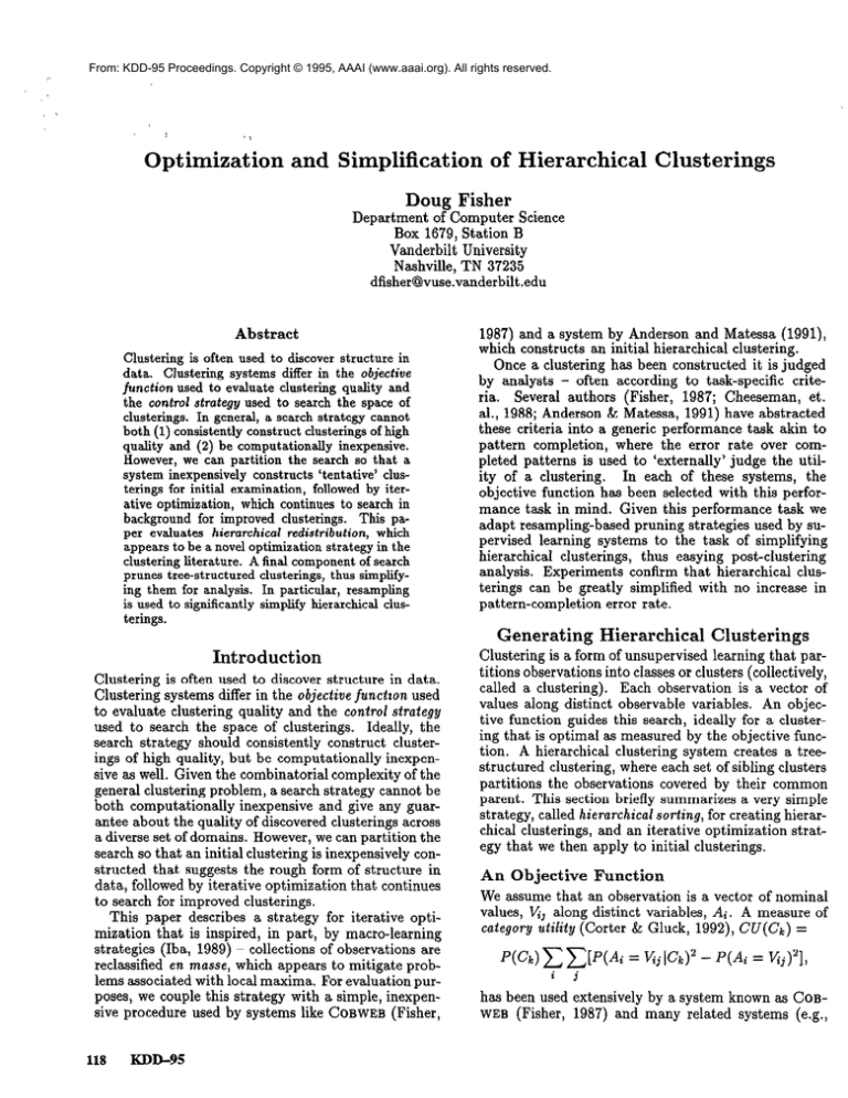
From: KDD-95 Proceedings. Copyright © 1995, AAAI (www.aaai.org). All rights reserved.
Optimization
and Simplification
of Hierarchical
Clusterings
Doug Fisher
Department of Computer Science
Box 1679, Station B
T,--J--L:ll
v mlaerullr TT-I-.---II-.
u nlverulby
Nashville, TN 37235
dfisher@vuse.vanderbilt.edu
Abstract
Clustering
is often used to discover structure
in
data. Clustering systems differ in the objective
function used to evaluate clustering quality and
the control strategy used to search the space of
clusterings. In general, a search strategy cannot
both (1) consistently construct clusterings of high
quality and (2) be computationally
inexpensive.
However, we can partition the search so that a
system inexpensively constructs ‘tentative’ clusterings for initial examination, followed by iterative optimization,
which continues to search in
background for improved clusterings.
This paper evaluates hierarchical redistribution,
which
appears to be a novel optimization strategy in the
clustering literature. A final component of search
prunes tree-structured clusterings, thus simplifying them for analysis. In particular, resampling
is used to significantly simplify hierarchical clusterings.
1987) and a system by Anderson and Matessa (1991),
which constructs an initial hierarchical clustering.
Once a clustering has been constructed it is judged
by analysts - often according to task-specific criteria. Several authors (Fisher, 1987; Cheeseman, et.
al., 1988; Anderson & Matessa, 1991) have abstracted
these criteria into a generic performance task akin to
pattern completion, where the error rate over completed patterns is used to ‘externally’ judge the utilIn each of these systems, the
ity of a clustering.
objective function has been selected with this nerformance task in mind. Given this performance task we
adapt resampling-based pruning strategies used by supervised learning systems to the task of simplifying
hierarchical clusterings, thus easying post-clustering
analysis. Experiments confirm that hierarchical clusterings can be greatly simplified with no increase in
pattern-completion
error rate.
Generating
Introduction
Clustering is often used to discover structure in data.
Clustering systems differ in the objective functzon used
to evaluate clustering quality and the control strategy
used to search the space of clusterings. Ideally, the
search strategy should consistently construct clusterings of high quality, but be computationally inexpensive as well. Given the combinatorial complexity of the
general clustering problem, a search strategy cannot be
both computationally inexpensive and give any guarantee about the quality of discovered clusterings across
a diverse set of domains. However, we can partition the
search so that an initial clustering is inexpensively constructed that suggests the rough form of structure in
&@
f~l1owe.d
hv
-J
itern.tive
-------
- r _ ------ - - - - -- t,hat
- nnt.imiaa.t,inn
cnnki~~es
to search for improved clusterings.
This paper describes a strategy for iterative optimization that is inspired, in part, by macro-learning
strategies (Iba, 1989) - collections of observations are
reclassified en masse, which appears to mitigate problems associated with local maxima. For evaluation purposes, we couple this strategy with a simple, inexpensive procedure used by systems like COBWEB (Fisher,
118
Km-95
Hierarchical
Clusterings
Clustering is a form of unsupervised learning that partitions observations into classes or clusters (collectively,
called a clustering). Each observation is a vector of
values along distinct observable variables. An objective function guides this search, ideally for a clustering that is optimal as measured by the objective function. A hierarchical clustering system creates a treestructured clustering, where each set of sibling clusters
partitions the observations covered by their common
parent. This section briefly summarizes a very simple
strategy, called hierarchical sorting, for creating hierarchical clusterings, and an iterative optimization strategy that we then apply to initial clusterings.
An Objective
Function
We assume that an observation is a vector of nominal
values, V& along distinct variables, Ai. A measure of
category uti1i-Q (Corter & Gluck, 1992), CV(Ck) =
has been used extensively by a system known as COB1987) and many related systems (e.g.,
WEB (Fisher,
Size
Shape
sma 0.50
squ 0.50
Color
blu 0.25
med 0.25
sph 0.50
gre 0.25
lar 0.25
P(root)=l.O
red 0.50
P(Cllroot)=0.50
sma 1.00
squ 1.00
blu 0.50
P(CZlroot)=0.50
med 0.50
sph 1.00
red 1.00
gre 0.50
sma 1.00
squ 1.00
blu 1.00
sma 1.00
squ 1.00
gre 1.00
P(C3~C1)=0.50
P(C41C1)=0.50
Figure 1: A probabilistic
Riawaa
YA”,VWY,
Wrsinhmrr
,,V’A-w---b,
& aa-,
T.i A””
10&i\A,.
.s,
Thje rr?egcr!:
rewg&
clusters, Ck, that increase the predictability of variable values within CI, relative to their predictability in
the population as a whole. This measure is similar in
form to the Gini Index, which has been used in supervised systems that construct decision trees (Weiss &
Kulikowski, 1991). The Gini Index typically measures
how well the values of a variable, Ai, predict a priorz
known class labels in a supervised context. The summation over Gini Indices reflected in CU addresses the
extent that a cluster predicts the values of all the variables. CU rewards clusters, Ck, that most reduce the
collective zmpwity over the variables.
In Fisher’s (1987) COBWEB system, the quality of
data
is
measured
by
partition
of
or the aver:v((c,,
a,. * .CN}) = Ck cU(ck)/N
age category utility of clusters in the partition.
The Structure
of Clusters
As in COBWEB,
AUTOCLASS (Cheeseman, et. al.,
1988), and other systems (Anderson & Matessa, 1991),
we will assume that clusters, ck, are described probabilistically: each variable value has an associated conditional probability, P(Ai = QICk), that reflects the
proportion of observations in ck that exhibit the value,
Ej, along variable Ai. In fact, each variable value is
actually associated with the number of observations
;,111 tha
“llcl
olrrotor
CIUUUL.L hmr;nm
“CY”“b
lar 0.50
th,t
UIIU” .ml..,.
“UIUCI,
nvnhnh;l;t;m
~‘““~U”XYLW
9-0
U&U PC.-CVLII-
puted ‘on demand’ for purposes of evaluation. In addition, there is a single root cluster, identical in structure
to other clusters, but covering all observations and containing frequency information necessary to compute
P(Ai = Q)‘s as required by category utility.
Figure 1 gives an example of a probablistic categorization
tree (i.e., hierarchical clustering) in which each node is
med 1.00
sph 1.00
red 1.00
lar 1.00
sph 1.00
red 1.00
P(C6lC2)=0.50
P(C51C2)=0.50
categorization
R.
- rlnnter
-_I_ 1--
tree.
nf
-_ nhnervatinns
----_
.-1_-_-
L qllmma.ri7w-l
L-----_----d--
nrohahilinticallv.
=--- ----- 1--I-_
~.
Observations are at leaves, and are described by three
variables: Size, Color, and Shape.
Hierarchical
Sorting
Our strategy for initial clustering is sorting. Given an
observation and a current partition, sorting evaluates
the quality of new clusterings that result from placing
the observation in each of the existing clusters, and
the quality of the clustering that results from creating
a new cluster that only covers the new observation; the
option that yields the highest quality score (e.g., using
PU) is selected. The clustering grows incrementally as
new observations are added.
This procedure is easily incorporated into a recursive loop that builds tree-structured clusterings: given
an existing hierarchical clustering, an observation is
sorted relative to the top-level partition (i.e., children
of the root); if an existing child of the root is chosen to include the observation, then the observation is
sorted relative to the children of this node, which now
serves as the root in this recursive call. When a leaf
is reached, the tree is extended downward. The maximum height of the tree can be bounded, thus limiting
downward growth to fixed depth.
This sorting strategy is identical to that used by Anderson and Matessa (1991). COBWEB (Fisher, 1987)
c,,.nmontn .nrt;nm
h.r
nnnpatnva
nf m~mn;n,n
mln’
UU~“%U~LUO
Y”‘UI’Sb
UJ “y.Au”“LY
“L
“Y”,~Y”sj,
u~‘
“‘“ff;mn
‘sYy,
and promotion. These operators combine, decompose,
and move clusters within a local region of a hierarchy each time an observation is sorted, if such changes
improve clustering quality. As many observations are
sorted, a cluster may migrate from one part of the
hierarchical clustering to another through the collective and repeated application of merging, splitting, and
Fisher
119
Figure 2: Hierarchical redistribution: the left subfigure indicates that cluster J has just been removed as a descendent of D and B, thus producing D’ and B’, and is about to be resorted relative to the children of the root (A).
The rightmost figure shows J has been placed as a new child of C.
promotion.
Unfortunately, these operators promote
very limited migration in practice. The experiments
of this paper do not use these operators in initial sorting, but the idea of moving clusters of observations en
masse inspires the strategy that we describe next.
Hierarchical
Redistribution
Hierarchical sorting constructs a tree-structured clustering cheaply, but this greedy procedure typically constructs nonoptimal clusterings. Thus, after an initial
clustering phase, a possibly offline process of iterative
optimization seeks to uncover better clusterings.
An iterative optimization
strategy that appears
novel in the clustering literature is iterative hierarchical redistribution.
It can be contrasted with a very
common strategy (e.g., Biswas, Weinberg, & Li, 1994)
of redistributing single observations: after initial clustering, observations may be moved one at a time from
one cluster to another, if to do so leads to an improved
clustering according to the objective function. However, redistributing observations one at a time is very
limited. In particular, the movement of an observation
may be required for the eventual discovery of a better
clustering, but the movement of any single observation
may initially reduce clustering quality, thus preventing the discovery of the better clustering. In response,
hierarchical redistribution considers the movement of
observation sets, represented by existing clusters in a
h;~~ronh;c..al
III~IWA\rlllticuI
ol.,.tm;nm
L..U”YQA111&.
Given an existing hierarchical clustering, an outer
recursive loop examines sibling clusters in the hierarchy in a depth-first fashion. For each set of siblings, an
inner, iterative loop examines each, removes it from its
current place in the hierarchy (along with its subtree),
and resorts the cluster relative to the entire hierarchy.
Removal requires that the various counts of ancestor
clusters be decremented. Sorting the removed cluster
120
KDD-95
is done based on the cluster’s probabilistic description,
and reauires a minor generalization of the procedure
for sort&g individual observations: rather than incrementing certain variable value counts by 1 at a cluster
to reflect the addition of a new observation, a ‘host’
cluster’s variable value counts are incremented by the
corresponding counts of the cluster (i.e., root of the
subtree) being classified. A cluster may return to its
original place in the hierarchy, or as Figure 2 illustrates, it (e.g., cluster J) may be sorted to an entirely
different location.
The inner loop reclassifies each sibling of a set, and
repeats until two consecutive iterations lead to the
same set of siblings. The outer loop then turns its
attention to the children of each of these remaining
siblings. Eventually, the individual observations represented by leaves are resorted (relative to the entire
hierarchy) until there are no changes from one iteration
to the next. The outer loop may make several passes
through the hierarchy until no changes occur from one
pass to the next.
In sum, hierarchical redistribution takes large steps
in the search for a better clustering. Similar to macrooperator learners (Iba, 1989) in problem-solving contexts, moving an observation set or cluster bridges distant points in the clustering space, so that a desirable
change can be made that would not otherwise have
been viewed as desirable if redistribution was limited
--AZC^
- ^_.^-,.-+ UI
,c iiiulvluual
* ~:..:A]..-1 uvwxvabwui5.
-L ^^__._A.:--- rnLbv uvvuut;ub
l.ne
reu1stribution of increasingly smaller, more granular clusters (terminating with individual observations) serves
to increasingly refine the clustering. In contrast to
COBWEB’S local application of operators such as merging, hierarchical redistribution considers more global
changes. In addition to COBWEB’S tree-restructuring
operators, hierarchical redistribution is related to treerestructuring strategies found in supervised, decision-
tree induction (Utgoff, 1994), and the general idea of
relocating observation sets more globally is found in a
recent clustering strategy by Nevins (1995).
Resultswith
Hierarchical
Redistribution
This section evaluates hierarchical redistribution:
a
random ordering of observations is generated and hierarchically sorted. Hierarchical redistribution is then
applied to the resultant hierarchical clustering. These
experiments assume that the primary goal of clustering is to discover a single-level partition of the data
that is of optimal quality. Thus, the objective function
score of the first-level partition is taken as the most
important dependent variable.
Table 1 shows results in 4 domains when the initial
tree constructed by sorting is bounded to be no more
than height 3 (i.e., the root has height 3, the leaves,
which are single observations, are height 0, and there
may be up to two levels of intermediate clusters). Row
one for each domain shows the PU scores of initial clusterings and the time (in seconds) required to construct
them.r Row two of each domain shows the PU scores
after hierarchical redistribution,
and the additional
time required for this optimization process. In general, hierarchical redistribution consistently improves
clustering quality in reasonable time. Fisher (1995)
c-lcw-rihea
-v-VIA”“”
nthm
..“-&“I
a-n,4mmt~
“dLy”~AA~A~““Y t.hat
“I&L,.” II)
ava111atn turn
“.CUIUUUI
V..” alWI-
ternative forms of iterative optimi\zsltion, (2) evaluate
optimization strategies using very ‘poor’ initial clusterings, and (3) evaluate clustering quality and the time
required for optimization as one varies the height of
the initial clustering. These experiments reveal that
hierarchical redistribution is robust across all these dimensions and is superior, with caveats, to the alternative optimization strategies examined. However, as
one increases height, there is negligible or no advantage
in terms of PU score on the domains examined, and
the cost of hierarchical redistribution rises significantly.
‘Thus, for reasons of cost, we adopt a tree construction
strategy that builds a hierarchical clustering three levels at a time (with hierarchical redistribution) in the
experiments of Section 3.
Hierarchical redistribution improves the results obtained with hierarchical sorting, but it may be appended to other greedy, hierarchical techniques as well,
such as agglomerative clustering methods.
Simplifying
Hierarchical
Clusterings
A hierarchical clustering can be grown to arbitrary
depth. if there is structure in the data, then ideaiiythe
top layers of the clustering reflect this structure (and
substructure as one descends the hierarchy). However,
lower levels of the clustering may not reflect meaningful structure. Inspired by certain forms of retrospective
pruning in decision-tree induction, we use resampling
‘Routines were implemented in SUN Common
compiled, and run on a SUN 3/60.
Lisp,
Table 1: Hierarchical redistribution with initial clusterings generated from sorting random ordered observations. Tree height is 3. Averages and standard devi-L:--~ 01I- r”v
nrr scores and Time (secondsj over 20 trials.
ations
Soybean/s
47obs,36vars
Soybean/l
307obs,36vars
House
435obs, lhars
Mushroom
1000obs.2?vars
I-c. --_L
sort
hier.
sort
hier.
sort
hier.
sort
h_ier:
PU score
1.53 (0.11)
1.62 (0.00)
0.89 (0.08)
1.07 (0.02)
1.22 (0.30)
1.68 (O.Oq
1.10 (0.13)
1:2? (Oi’-‘Oj
Time
18.3 (1.8)
93.8 (27.5)
142.4 (10.2)
436.3 (138.9)
104.3 (8.7)
355.0 (71.1)
406.6 (64.2)
12sgi2 (4.58)
to identify ‘frontiers’ of a hierarchical clustering that
are good candidates for pruning. Following initial hierarchy construction and iterative optimization, this
simplification process is a final phase of search through
the space of hierarchical clusterings that is intended to
ease the burden of a data analyst.
Identifying
Variable Frontiers
4fino...--1
~--Lx
ITT%’
1
3everai autnors \r isner, lYu I ; Cheeseman, et.
ai.,
1988; Anderson & Matessa, 1991) motivate clustering
as a means of improving performance on a task akin
to pattern completion, where the error rate over completed patterns can be used to ‘externally’ judge the
utility of a clustering. Given a probabilistic categorization tree, a new observation with an unknown value for
a variable can be classified down the hierarchy using
a small variation on the hierarchical sorting procedure
described earlier. Classification is terminated at an existing node (cluster) along the classification path, and
the variable value of highest probability at that cluster is predicted as the unknown variable value of the
new observation. Naively, classification might always
terminate at a leaf (i.e., an observation), and the leaf’s
value along the specified variable would be predicted
as the variable value of the new observation. However,
a variable might be better predicted at some internal
node in the classification path. We adapt retrospective
pruning strategies in decision tree induction, such as
reduced error pruning (Quinlan, 1987), to the task of
identifying these internal nodes.
Given a hierarchical clustering and a validation set
-I -L _^__._LZ--- AL-.-l:,-L:...
~-I rUL UUS~:TV~LIOIIS~
bne vallaaGion se6 is used to identify
an appropriate frontier of clusters for prediction of
each variable. Figure 3 illustrates that the preferred
frontiers of any two variables may differ, and clusters
within a frontier may be at different depths. For each
variable, Aa, the objects from the validation set are
each classified through the hierarchical clustering with
the value of variable Ai ‘masked’ for purposes of classification. At each cluster encountered during classifica-
Fisher
121
-3
Figure 3: Frontiers for three variables in a hypothetical
tion the observation’s value for Ai is compared to the
most probable value for Ai at the cluster; if they are
the same, then the observation’s value would have been
correctiy predicted at the ciuster. A count of aii such
correct predictions for each variable at each cluster is
maintained.
Following classification for all variables
over all observations of the validation set, a preferred
frontier for each variable is identified that maximizes
the number of correct counts for the variable.
The identification of variable-specific frontiers facilitates a number of pruning strategies. For example,
a node that lies below the frontier of every variable
offers no advantage in terms of pattern-completion
error rate; such a node probably reflects no meaningful
structure
---.-.---__ I-, mav
_._..~ be
- _ nruned.
=----- -.
-__- _.-_- and
..__- it-. fand
\----- its
--- descendentsj
However, if an analyst is focusing attention on a subset
of the variables, then frontiers might be more flexibly
exploited for pruning.
The novelty of the validation strategy described here
stems from an observation that any single partition
of observations may overfit the data relative to some
variables and underfit relative to others. Undoubtedly,
the identification of variable-specific frontiers can also
be implemented by adapting Bayesian or hypothesistesting techniques, which are currently used to terminate hierarchical decomposition by identifying a single,
11..
.
variable-independent
frontier (e.g., hrToCLAss j.
of A3
clustering.
Table 2: Characteristics of optimized clusterings before
and after validation. Average and standard deviations
nvo,
V.Ih
311
I” t.ria1n
“IIWI”.
Soy/s
Soy/l
House
Leaves
Accuracy
Frontrer
Leaves
Accuracy
IFrontier
Leaves
Accuracy
pI”II”lsLI
‘rc.nC.ar
Unvalidated
18.00 (0.00)
0.85 (0.01)
18.00 0.00
122.00 (0.00)
0 83 (0 02)
122.00 (0.00)
174.00 (0.00)
0.76 (0.02)
174.00 (0.00)
Validated
13.10 (1.59)
0 85 (0 01)
2:75 (1:17)
79.10 (5.80)
083 (002)
17.01 (4.75)
49.10 (7.18)
0.81 (0.01)
9.90 (5.16)
.
To test the validation procedure’s promise for simplifying hierarchical clusterings, each of the data sets used
in the experiments of Section 2.5 was randomly divided into three subsets: 40% for training, 40% for
validation, and 20% for test. A hierarchical clustering
is first constructed by sorting the training set. This hierarchy is then optimized using hierarchical redistribution. The final hierarchy decomposes the training set
During testing of a validated clustering, each variable of each test observation is masked in turn. When
classification reaches a cluster on the frontier of the
masked variable, the most probable value is predicted
as the value of the observation; the proportion of correct predictions for each variabie over the test set is
recorded. For comparative purposes, we also use the
test set to evaluate predictions stemming from the unvalidated tree, where all variable predictions are made
at the leaves (singleton clusters) of this tree.
Table 2 shows results from 20 experimental trials
using unvalidated and validated clusterings. The first
row of each domain lists the average number of leaves
for the unvalidated and validated trees.
The unvalidated clusterings decompose the training data to
single-observation leaves - the number of leaves equals
to
&daton
1- L--o--1--
the
Experiments
with
cil&ers.
Validation
7 e;t.ch
-----
c~nt,ainin~
D A.
- single
----
training
observation. The validation set is then used to identify
variable frontiers within the entire hierarchy.
122
KDD-95
~~~~~~~~ nf irainina b nhmwntinna
Y-Y”* IVYIVYY.
Tn the
II&
“Al” xralic-lat~rl
.U11UUUYU
clustering, we assume that clusters are pruned if they
lie below the frontiers of all variables. Thus, a leaf in a
validated clustering is a cluster (in the original clustering) that is on the frontier of at least one variable, and
none of its descendent clusters (in the original clustering) are on the frontier of any variable.
Prediction accuracies in the second row of each domain entry are the mean proportion of correct predictions over all variables over 20 trials. Predictions
were generated at leaves (singleton clusters) in the unvalidated hierarchical clusterings and at appropriate
variable frontiers in the validated clusterings. In all
cases, validation/pruning
substantially reduces clustering size and it does not diminish accuracy.
We have suggested that more flexible pruning or ‘attention’ strategies might be possible when an analyst
is focusing on one or a few variables. We will not specify such strategies, but the statistic given in row 3 of
each domain entry suggests that clusterings can be rendered in considerably simpler forms when an analyst’s
attention is selective. Row 3, labeled IFrontier/, is the
average number of frontier clusters per variable. This
is an average over all variables and all experimental
trials. Intuitively, a frontier cluster of a variable is a
‘leaf’ as far as prediction of that variable is concerned.
The IFrontier entry for unvalidated clusterings is simply given by the number of leaves, since this is where all
variable predictions are made in the unvalidated case.
Our results suggest that when attention is selective, a
partial clustering that captures the structure involving selected variables can be presented to an analyst
in very simplified form.2
Concluding
Remarks
Error rate and simplicity are objective criteria, with
analogs in supervised (e.g., decision-tree) induction,
that can be used to evaluate the merits of differing
objective functions.
The relation between the Gini
Index and Category Utility suggests that other objective functions can be derived from analog selection
measures (e.g., Lopez de Mantaras, 1991) of decision
tree induction (Fisher, 1995). However, our focus has
not been on objective functions, but on search control strategy; the search for hierarchical clusterings
can be partitioned into three phases: (1) inexpensive
generation of a hierarchical clustering for initial examination, (2) iterative optimization for clusterings of
better quality, and (3) retrospective simplification of
generated clusterings. In particular, the paper introduces apparently novel (but derivative) implementations of phases 2 and 3. These are an iterative optimization strategy called hierarchical redistribution,
which relocates observation sets en masse, and pruning/simplification
strategies based on the identification
of variable-specific frontiers. For purposes of evaluation we have coupled these with a particular objective
2Fisher (1995) also looks at the relative amount of simplification that can be performed with optimized (using
hierarchical redistribution) and unoptimized clusterings.
function, initial clustering strategy, and data representation. These two strategies, however, may be coupled
with other initial clustering strategies, objective functions, and (e.g., numeric) data representations as well
(Fisher, 1995).
Acknowledgements
This work was supported by
grant NAG 2-834 from NASA Ames Research Center.
References
Anderson, J. R., & Matessa, M. (1991). An interative
Bayesian algorithm for categorization. In D. Fisher
& M. Pazzani (Eds.), Concept formation:
Knowledge and experience in unsupervised learning. San
Mateo, CA: Morgan Kaufmann.
Biswas, G., Weinberg, J., & Li, C. (1994). ITERATE:
A conceptual clustering method for knowledge discovery in databases. In B. Braunschweig and R. Day
(Eds.) Innovative Applications of Artificial Intelligence in the Oil and Gas Industry. Editions Technip.
Cheeseman, P., Kelly, J., Self, M., Stutz, J., Taylor,
W., & Freeman, D. (1988). AutoClass: A Bayesian
classification system. Proceedings of the Fifth International Machine Learning Conference (pp. 54-64).
Ann Arbor, MI: Morgan Kaufmann.
Corter, J., & Gluck, M. (1992). Explaining basic categories: feature predictability and information. Psychological Bulletan, 111, 291-303.
Fisher, D. H. (1987). Knowledge acquisition via incremental conceptual clustering. Machine Learning,
2, 139-172.
Fisher, D. H. (1995). Iterative optimization and simplzjkatzon of hierarchical clusterings. Technical Report CS-95-01, Department of Computer Science,
Vanderbilt University, Nashville, TN.
Iba, G. (1989). A h euristic approach to the discovery
of macro operators. Machzne Learning, 3, 285-317.
Lopez de Mantaras, R. (1991). A distance-based attribute selection measure for decision tree induction.
Machine Learning, 6, 81-92.
Nevins, A. J. (1995). A branch and bound incremental clusterer. Machzne Learning, 18, 1, 5-22.
Quinlan, J. R. (1987). Simplifying decision trees.
International Journal of Man-machine Studies, 2’7,
221-234.
Utgoff, P. (1994). A n improved algorithm for incremental induction of decision trees, Proceedings of
the Eleventh International Conference on Machine
Learning (pp. 318-325). New Brunswick, NJ: Morgan Kaufmann.
Weiss, S., & Kulikowski, C. (1991). Computer Systems that Learn. San Mateo, CA: Morgan Kaufmann Publishers.
Fisher
123