From: KDD-98 Proceedings. Copyright © 1998, AAAI (www.aaai.org). All rights reserved.
An enhanced representation of time series which allows fast and accurate
classification, clustering and relevance feedback
Eamonn J. Keogh and Michael J. Pazzani
Departmentof Information and ComputerScience
University of California, Irvine, California 92697USA
{ eamonnpazzani}@ics.uci.edu
Abstract
We introduce an extendedrepresentationof time seriesthat
allows fast, accurateclassificationand clusteringin addition
to the ability to explore time series data in a relevance
feedbackframework. The representationconsistsof piecewise linear segmentsto representshapeand a weight vector
that contains the relative importance of each individual
linear segment.In the classificationcontext, the weightsare
learned automatically as part of the training cycle. In the
relevancefeedbackcontext, the weights are determinedby
an interactive and iterative process in which users rate
various choices presented to them. Our representation
allows a user to define a variety of similarity measuresthat
can be tailored to specific domains. We demonstrateour
approachon spacetelemetry,medical and syntheticdata.
1.0 Introduction
Time series account for much of the data stored in
business, medical, engineering and social science
databases.Much of the utility of collecting this data comes
from the ability of humans to visualize the shape of the
(suitably plotted) data, and classify it. For example:
Cardiologists view electrocardiograms to diagnose
l
arrhythmias.
Chartists examine stock market data, searching for
certain shapes, which are thought to be indicative of
a stock’s future performance.
Unfortunately, the sheer volume of data collected means
that only a small fraction of the data can ever be viewed.
Attempts to utilize classic machine learning and
clustering algorithms on time series data have not met with
great success. This, we feel, is due to the typically high
dimensionality of time series data, combined with the
difficulty of defining a similarity measure appropriate for
the domain. For an example of both these difficulties,
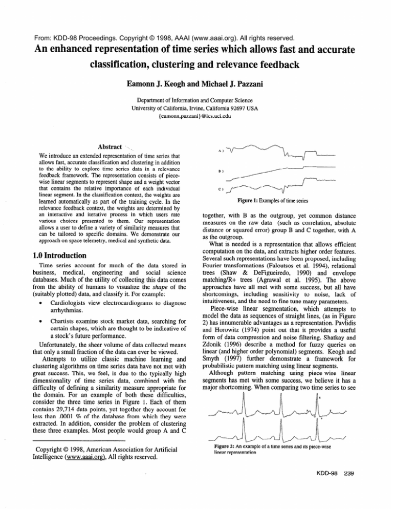
consider the three time series in Figure 1. Each of them
contains 29,714 data points, yet together they account for
less than .OOOl % of the database from which they were
extracted. In addition, consider the problem of clustering
these three examples. Most people would group A and C
l
Copyright 0 1998, American Association for Artificial
Intelligence (www.aaai.orn), All rights reserved.
Figure
1:
Examples
of timeseries
together, with B as the outgroup, yet common distance
measures on the raw data (such as correlation, absolute
distance or squared error) group B and C together, with A
as the outgroup.
What is needed is a representation that allows efficient
computation on the data, and extracts higher order features.
Several such representations have been proposed, including
Fourier transformations (Faloutsos et al. 1994), relational
trees (Shaw & DeFigueiredo, 1990) and envelope
matching/R+ trees (Agrawal et al. 1995). The above
approaches have all met with some success, but all have
shortcomings, including sensitivity to noise, lack of
intuitiveness, and the need to fine tune many parameters.
Piece-wise linear segmentation, which attempts to
model the data as sequences of straight lines, (as in Figure
2) has innumerable advantages as a representation. Pavlidis
and Horowitz (1974) point out that it provides a useful
form of data compression and noise filtering. Shatkay and
Zdonik (1996) describe a method for fuzzy queries on
linear (and higher order polynomial) segments. Keogh and
Smyth (1997) further demonstrate a framework for
probabilistic pattern matching using linear segments.
Although pattern matching using piece-wise linear
segments has met with some success, we believe it has a
major shortcoming. When comparing two time series to see
Figure 2: An example
of a timeseriesandits piece-wise
linear representation
KDD-98
239
if they are similar, all segments are considered to have
equal importance. In practice, however, one may wish to
assign different levels of importance to different parts of
the time series. As an example, consider the problem of
pattern matching with electrocardiograms. If a cardiologist
is attempting to diagnose a recent myocardial infarction
(MI) she will pay close attention to the S-T wave, and
downplay the importance of the rest of the
electrocardiogram. If we wish an algorithm to reproduce
the cardiologist’s ability, we need a representation that
allows us to weight different parts of a time series
differently.
In this paper, we propose such a representation. We use
piece-wise linear segments to represent the shape of a time
series, and a weight vector that contains the relative
importance of each individual linear segment.
2.0 Representation of time series
There are numerous algorithms available for segmenting
time series, many of which where pioneered by Pavlidis
and Horowitz (1974). An open question is how to best
choose K, the ‘optimal’ number of segments used to
represent a particular time series. This problem involves a
trade-off between accuracy and compactness, and clearly
has no general solution. For this paper, we utilize the
segmentation algorithm proposed in Keogh (1997).
2.1 Notation
For clarity we will refer to ‘raw’, unprocessed temporal
data as time series, and a piece-wise representation of a
time series as a sequence. We will use the following
notation throughout this paper. A time series, sampled at k
points, is represented as an uppercase letter such as A. The
segmented version of A, containing K linear segments, is
denoted as a bold uppercase letter such as A, where A is a
5tuple of vectors of length K.
A= { AxL,AxR,AYL,AYR,Aw}
The i* segment of sequence A is represented by the line
between (AxL, AYL,) and (AxR, AYR,), and Aw,, which
represents the segments weight. Figure 3 illustrates this
notation.
t
2.2 Comparing time series
An advantage in using the piece-wise linear
segment representation is that it allows one to define a
variety of distance measures to represent the distance
between two time series. This is important, because in
various domains, different properties may be required of a
distance measure. Figure 4 shows some of the various
distortions one can encounter in time series.
m
m
m-
Noise
Discontinuities
Figure 4: Some of the difficulties encountered in defining a distance measure
for time series
It is possible to define distance measures for sequences
that are invariant to any subset of the illustrated distortions.
For the experiments in this paper we used the simple
distance measure given below. This measure is designed to
be insensitive to offset translation, linear trends and
discontinuities.
D(A,B>=C;,Ay
*By
*I(AYL, - BY&)-(AYR,-BYRJ
It is convenient for notational purposes to assume that
the endpoints of the two sequences being compared are
aligned. In general, with real data, this is not the case. So
we will have to process the sequences first, by breaking
some segments at a point which corresponds to an endpoint
in the other sequence. This can be done in O(K).
Ff
11-1
Figure 3: We represent times series b a sequence of straight se ments,
together with a sequence of weights (si own as the histogram) w 8.lch contain
the relative importance of each segment
After a time series is segmented to obtain a sequence, we
initialize all the weights to one. Thereafter, if any of the
weights are changed, the weights are renormalized such
that the sum of the products of each weight with the length
of its corresponding segment, equals the length of the
entire sequence, so that the following is always true:
c;,Wi
240
Keogh
*(Ax&
-AxL,)=AxR,
-AxL,
Figure 5: An example of time series hierarchically clustered using our
distance measure
2.3 Merging time series
In this section we define an operation on sequences
which we call ‘merge’, The merge operator allows us to
combine information from two sequences, and repeated
application of the merge operator allows us to combine
information from multiple sequences. The basic idea is that
the merge operator takes two sequences as input, and
returns a single sequence whose shape is a compromise
between the two original sequences, and whose weight
vector reflects how much corresponding segments in each
sequence agree.
When merging sequences one may wish for one of the
two input sequences to contribute more to the final
sequence than the other does. To accommodate this, we
associate a term called ‘influence’ with each of the input
sequences. The influence term associated with a sequence
S is a scalar, denoted as SI, and may be informally
considered a ‘mixing weight’. Where the influence term
comes from depends on the application and is discussed in
detail in sections 3.1 and 4.1 below.
To merge the two sequences A and B with influence
terms AI and BI respectively, we use the following
d algorithm that creates the sequence C:
sign = -1
if (AI * BI < 0) then
sign = 1
else
end
/ max(lAI[,IB~l)
mw = min(lAII,jBI()
scale = max(max(AyL), (AYR) )- min(min(AyL),
for
i = 1 to K
CXLi = AxLi
CXRi = AXRi
CYL~= ( (AYL~ * AI)+(BYL~ * BI))/(AI+BI)
CYR~= (( AYR~ * AI)+(BYR~ * BI) )/(AI+BI)
run
= AXRi - AXl,
rise
= ~(AYL~BYL~)- (AYR~- BYRD) 1
d
= (rise / run) * scale
Cw, = (Aw,*Bw,)* (l+(sign
* mag)/ (1
end
Cw = normalize(Cw)
(AYR))
+ d))
Table 1: The merge algorithm
2.4 Learning prototypes
Although the merge operator is designed to be a
component in the more sophisticated algorithms presented
below, it can, by itself, be considered a simple learning
algorithm that creates a prototypical sequence. Creating a
prototype solely from positive examples works in the
following manner. We have a model sequence A, which is
a typical example of a class of sequences. If we merge
sequence A with sequence B, another member of the same
class, the resultant sequence C can be considered a more
general model for the class. In particular the differences in
shape are reduced by averaging, and the weights for similar
segments are increased.
In contrast, creating a prototype from both positive and
negative examples uses a negative influence for the
negative examples. As before, suppose we have a sequence
A, which is an example of one class of sequences.
However, suppose B is an example of a different class. If
we merge A with B, using a negative influence term for B,
the resultant sequence C is a new prototype for A’s class
where the differences in shape between A and B are
exaggerated and the weights for similar segments are
decreased.
The above maps neatly to our intuitions. If we are
learning a prototype for a class of sequences from a set of
positive examples, we want the shape learned to be an
average of all the examples, and we want to increase the
weight of segments that are similar, because those
segments are characteristic of the class. If however, we are
trying to learn from a negative example, we want to
exaggerate the differences in shape between classes, and
decrease the weight of similar segments, because segments
that are similar across classes have no discriminatory
power.
3.0 Relevance feedback
Relevance feedback is the reformulation of a search
query in response to feedback provided by the user for the
results of previous versions of the query. It has an
extensive history in the text domain, dating back to
Rocchio’s classic paper (1971). However, no one has
attempted explore time series databases in a relevance
feedback framework, in spite of the fact that relevance
feedback has been shown to significantly improve the
querying process in text databases (Salton & Buckley,
1990). In this section we present a simple relevance
feedback algorithm which utilizes our representation and
we demonstrate it on a synthetic dataset.
Our relevance feedback algorithm works in the
following manner. An initial query sequence Q is used to
rank all sequences in the database (this query may be hand
drawn by the user). Only the best n sequences are shown
to the user. The user assigns influences to each of n
sequences. A positive influence is given to sequences that
the user approves of. Negative influences are given to
sequencesthat the user finds irrelevant.
The relative magnitude of influence terms reflects how
strongly the user feels about the sequences. So if a user
“likes” Si twice as much as Sj he can assign influences of
1,s or 2,1 etc. The sequences are then merged to produce a
new query, and the process can be repeated as often as
desired.
t [S,,S,Il
Qll.2”= merge ( [Qold,Q,,,Il, [S,,S,Il
Q,,I = QolaI + S,I + S,I + . . + SJ
I..., [S,,S,Il
1
3.1 Experimental results
To test the above algorithm, we conducted the following
experiment. We constructed 500 “Type A”, and 500 “Type
B” time series, which are defined as follows:
0
0
Type A: Sin(x’> normalized to be between zero and
one, plus Gaussian noise with CJ= .l
-25x52
Type B: Tan(Sin(x3)) normalized to be between zero
and one, plus Gaussian noise with 0 = .l -2 I x I 2
KDD-98
241
4.0 Classification
Tan(Sin(x3))
Sin(x3)
Given our representation, an obvious approach to
classification is to merge all positive instances in the
training set, and use the resultant sequence as a template to
which the instances to be classified are compared. This
may work in some circumstances, but in some domains it
may totally fail. The reason for the potential failure is that
there may be two or more distinct shapes that are typical of
the class.
To avoid this problem, an algorithm needs to be able to
detect the fact that there are multiple prototypes for a given
class, and classify an unlabeled instance to that class if it is
sufficiently similar to any prototype. In the next section we
describe such an algorithm, which we call CTC (Cluster,
Then Classify).
A)
B)
c>
Figure
A)
B)
Cl
6: Synthetic data created for relevance feedback experiment
The original time series.
The original time series with noise added.
The segmented version of the time series.
Twenty-five experimental runs were made. Each run
consisted of the following steps. A coin toss decided
whether Type A or Type B was to be the “target” shape
(that is, the shape to be considered “relevant” for that
particular experiential run). The initial query was made,
and the quality of the ranked sequences was measured as
defined below. The best 15 sequences were shown to the
user, who then rated them by assigning influences that
reflected how closely he thought they resembled the target
shape. A new query was built and the search/rate process
was repeated twice more.
We evaluated the effectiveness of the approach by
measuring the average precision of the top 15 sequences,
and the precision at the 25, 50 and 75 percent recall points.
Precision (P) is defined as the proportion of the returned
sequences which are deemed relevant, and recall (R) is
defined as the proportion of relevant items which are
retrieved from the database. These results are shown in
Table 2.
In order to see if the ability to assign negative influence
terms is helpful, we did the following. For each
experimental run we also built queries which contained just
the feedback from the sequences judged relevant. These
results are shown in parentheses in Table 2.
Initial
Poftop
15
Pat25%R
PatSO%R
1 Pat75%R
1
Query
Second Query
.51
.91
.52
.49
.91 (.69)
-89 (661
.87 (.63)
.51
(.68)
Third Query
.97
(.72)
.96 (.71)
.95 f.691
.95 (.68)
Table 2: Results of relevance feedback experiments. The values recorded in
parentheses are for the queries built just from positive feedback
As one might expect, the initial query (which does not
have any user input) returns the sequences in essentially
random order. The second query produces remarkable
improvement, and the third query produces near perfect
ranking. The queries built from just positive feedback do
produce improvement, but are clearly inferior to the more
general method. This demonstrates the utility of learning
from both positive and negative instances.
4.1 Classification algorithm
Table 3 shows an outline of our learning algorithm. The
input is S, the set of n sequencesthat constitute the training
data. The output is P, a set of sequences, and a positive
scalar E.
An unseen sequence U will be classified as a member of
a class if and only if, the distance between U and at least
one member of P is less than E.
The algorithm clusters the positive examples using the
group average agglomerative method as follows. The
algorithm begins by finding the distance between each
negative instance in S, and its closest positive example.
The mean of all these distances, neg-dis, is calculated. Next
the distance between each positive instance in S, and the
most similar positive example is calculated. The mean of
all these distances, pos-dis, is calculated. The fraction q1 =
pos-dis, /neg-dis, can now be calculated.
At this point, the two closest positive examples are
replaced with the result of merging the two sequences,and
the process above is repeated to find the fraction q2 = posdis, / neg-dis,. The entire process is repeated until a single
sequence remains. Figure 7 shows a trace through this part
of the algorithm for a dataset that contains just 4 positive
instances. The set of sequences returned is the set for
which q1is minimized.
The E returned is (pas-dis, + neg-dis,) /2.
Let Pi be the set of all positive
instances
in S
Cluster
all sequences in Pi
for
i = 1 to n
neg-dis,
= mean distance
between all negative
instances
and their
closest
match in Pi
pos-dis,
= mean distance
between all positive
instances
and their
closest
match in Pi
qi= pos-dis i / neg-dis,
Let A and B be the closest
pair of sequences in Pi
C = merge([A,AIl,
[B,BII)
CI = AI + BI
Remove A and B from Pi
Add C to Pi
end
let best equal the i for which qI is minimized
return
P,., , (pas-dis,,
+ neg-dis,,,,)
/ 2
Table 3: The CTC learning algorithm
242
Keogh
4.2 Experimental results
To test the algorithm presented above we ran
experiments on the following datasets.
l
Shuttle: This dataset consists of the output of 109
sensors from the first eight-hours of Space Shuttle
mission STS-067. The sensors measure a variety of
phenomena. Eighteen of them are Inertia Movement
Sensors, measured in degrees (examples are shown
in Figures 1 and 7). The task is to distinguish these
from the other 91 sensors.
l
Heart: This dataset consists of RR intervals
obtained form Holter ECG tapes sampled at 128 Hz
(Zebrowski 1997). The data is in a long sequence
that contains 96 ventricular events. We extracted the
96 events, and 96 other sections, of equal length,
chosen at random.
For comparison purposes we evaluated 4 algorithms on
the two datasets described above. CTC is the algorithm
described in section 4.1. CTCuw is the same algorithm
with the weight feature disabled (we simply hardcoded the
weights to equal one). NN is a simple nearest neighbor
algorithm that uses the raw data representation of the time
series. An unlabeled instance is assigned to the same class
as its closest match in the training set. We used absolute
error as a distance measure, having empirically determined
that it was superior to the other obvious candidates (i.e.
squared error, correlation). NNs is the same algorithm as
NN except it uses the sequence representation and the
distance measure defined in section 2.2.
We ran stratified 10 fold cross validation once. All
algorithms were trained and tested on exactly the same
folds. The results are presented in table 4.
Shuttle
Heart
CTCuw
96.0
69.1
CTC
100
85.6
Table 4: Experiment
NN
82.1
59.8
results of classification
NNs
89.3
64.6
Default
83.5
50.0
experiments
On both datasets the CTC algorithm performs the best.
Its ability to outperform CTCuw seems to be a justification
of our weighted representation. On the Shuttle dataset NN
performs at the base rate. We surmise this is probably due
to its sensitivity to discontinuities, which are a trait of this
dataset. NNs ability to do significantly better supports this
hypothesis.
P2
q~= .63
9
q2= .52
5.0 Related work
There has been no work on relevance feedback for time
series. However, in the text domain there is an active and
prolific research community. Salton and Buckley (1990)
provide an excellent overview and comparison of the
various approaches.
6.0 Conclusions
We introduced a new enhanced representation of time
series and empirically demonstrated its utility for
clustering, classification and relevance feedback.
References
Agrawal, R., Lin, K. I., Sawhney,H. S., & Shim, K.(1995). Fast
similarity searchin the presenceof noise, scaling, and translation
in times-seriesdatabases.In VLDB, September.
Faloutsos,C., Ranganathan,M., & Manolopoulos, Y. (1994).
Fast subsequencematching in time-seriesdatabases.SIGMOD Proceedingsof Annual Conference,Minneapolis,May.
Hagit, S., & Zdonik, S. (1996). Approximate queries and
representationsfor large data sequences. Proc. 12th IEEE
International Conferenceon Data Engineering.pp 546-553,New
Orleans,Louisiana,February.
Keogh, E. (1997). Fast similarity search in the presence of
longitudinal scaling in time seriesdatabases.Proceedingsof the
9th InternationalConferenceon Tools with Artificial Intelligence.
pp 578-584.IEEE Press.
Keogh, E. & Smyth, P. (1997). A probabilistic approachto fast
patternmatchingin time seriesdatabases.Proceedingsof the 3’d
International Conference of Knowledge Discovery and Data
Mining. pp 24-20, AAAI Press.
Pavlidis,T. & Horowitz, S. (1974). Segmentationof plane curves.
IEEE Transactionson Computers,Vol. C-23, No 8.
Salton, G., & Buckley, C. (1990). Improving retrieval
performanceby relevancefeedback.JASIS 41. pp. 288-297.
Shaw, S. W. & DeFigueiredo, R. J. P. (1990). Structural
processing of waveforms as trees. IEEE Transactions on
Acoustics,Speech,and Signal Processing.Vol. 38 No 2 February.
Rocchio, J. J., Jr.(1971). Relevance feedback in information
retrieval: The Smart System - Experiments in Automatic
DocumentProcessing.Prentice-HallInc., pp. 337-354.
Zebrowski,J,J. (1997).
http://www.mpipks-dresden.mpg.de/~ntptsa/Data/Zebmwski-D/
P4
P3
P--q3= .21
q4= .47
Figure 7: A trace through the CTC algorithm on a small dataset. The first set of prototypes PI, are too specific and do not generalize to the test set. The
final set P4 contains a single sequence that is too general, because it is trying to model two distinct shapes. The set P3 is the best compromise.
KDD-98
243
Related
Work.
Brin et al. (Brin, Motwani, & Silverstein 1997) used the chi-squared test to look for correlated associations, but did not take into account the
number of hypotheses were being tested. PiatetskyShapiro (Piatetsky-Shapiro 1991) had a similar idea
when he argued that a rule X + Y is not interesting if support(X * Y) N support(X) x support(Y),
but again did not consider the number of hypotheses.
2. Statistical
Significance
Rules
of Association
In this section, we discuss issues of statistical signifi-
cance of a set of association rules. First, in Section 2.1,
we discuss the statistical significance of a single rule.
However, when we analyze many rules simultaneously,
the significance test has to take into account the number of hypotheses being tested. This is the so-called
multiple comparisons problem (Hochberg & Tamhane
1987). Typically the test statistics corresponding to
the hypotheses being tested are not independent. It
is important to observe that the number of hypotheses implicitly being tested may be much greater than
the number of output rules; we give an upper bound for
this number in Section 2.2. This bound may, in general,
be too conservative. We offer a practical way of dealing with this problem in Section 2.3; the idea is to use
resampling to determine a good acceptance threshold.
Finally, in Section 2.4, we describe the computation of
confidence intervals for the support and confidence of a
rule.
2.1. Statistical
Association
Significance
of a Single
We view a dataset consisting of n transactions as the realizations of n independent identically distributed random boolean vectors, sampled from the “real world”
distribution. Let 7rs denote the “real world” probability
that a transaction contains a given itemset S. Thus, the
number of transactions NS in the sample (i.e., dataset)
that contain S is a binomial random variable with success probability 7r = ns and n trials.
Hypothesis
testing
and minimum
support.
The
minimum support requirement can be cast in the hypotheses testing framework as follows. For example,
suppose our minimum support requirement is 10%. For
each itemset S, let Hf be the null hypothesis that
ns = 0.1, and let us test it against the crlternative hypothesis H& that ns > 0.1. Let ps be the fraction of
transactions in the dataset that contain S. The test is
to compare ps with a threshold value po and reject H:
if and only if ps 2 pc. There are two kinds of possible
errors (Cryer & Miller 1994):
~~
The selection of ps is determined by a bound on the
desired probability of Type I error, which is called the
significance level.
P-values.
In general, the p-value of a test result is the
probability of getting an outcome at least as extreme as
the outcome actually observed; the p-value is computed
under the assumption that the null hypothesis is true
(Cryer & Miller 1994). In our example, the p-value
corresponding to an observed fraction ps is equal to the
probability, under the assumption that rs = 0.1, that
the fraction of transactions that contain S is greater
than or equal to ps.
In order to compute the p-value, we use either the
normal approximation, the Poisson approximation, or
the exact binomial distribution, depending on the actual values of n, the minimum support requirement,
and the observed support. For example, suppose n =
10,000, the minimum support is 7r = 0.1 and the observed support is p = 0.109. We use the normal approximation. The mean is 7r = 0.1, and the standard
deviation is J(r( 1 - n)/n) = J(O.O9/10000) = 0.003.
Since p is three standard deviations greater than 7rTT,
the
p-value is 0.0013.
Testing
Independence.
Consider an association
rule S 3 T, where S and T are sets of items. As a null
hypothesis we assume that S and 2’ occur in transactions independently. Thus, under the null hypothesis,3
,$hT = *TT’x nT. As an alternative hypothesis, we can
use the inequality nShT > ns x nT, which means that
the conditional probability of T given S is greater than
the probability of T.
If the values 7rs and rT are assumed to be known
with sufficient accuracy, we can use the value ns x nT to
compute a p-value for S + 2’. This p-value corresponds
to the probability, under the assumption that S and 2’
are independent, that the empirical frequency of the
set S U T will be greater than pSAT. Since we don’t
know the actual values of rs and 7rT, we use ps and
‘We denote the event that S U T is included in the transaction by S A 2’ since this is indeed the intersection of the
events corresponding to S and T.
KDD-98
275
pT (the fractions of transactions that contain S and T,
respectively) as estimates for ns and rT. The lower
the p-value, the more likely it is that S and T are not
independent.
2.2. Statistical
Associations
Significance
of a Set of
Suppose we are testing k null hypotheses Hi, . . . , Ht ,
and denote by qi the probability of rejecting Hi when
it is true. The probability of rejecting at least one of
the null hypotheses when they are all true is at most
q1 + * * e+ qk. Thus, if we wish the latter to be smaller
than, say, 0.05, it suffices to determine thresholds for
the individual tests so that q; < 0.05/k. This bound
may be very small if the number of hypotheses implicitly being tested is very large. Indeed, since under
the null hypothesis the empirical p-value is distributed
uniformly, when we test k true null hypotheses whose
test statistics are independent random variables, the
expected value of the smallest p-value is l/(k + l), so
in order to achieve a small probability of rejecting any
true null hypothesis we would have to choose thresholds
even smaller than that. Note that when we test independence of pairs in a set of, say, 10,000 items, then the
value of k would be greater than 107.
Obviously, if we wish to achieve a good probability of
rejecting most “false discoveries”, we have to increase
the probability of rejecting some true ones as well. In
other words, when we attempt to discover more true
rules, we also increase the risk of false discoveries (i.e.,
rejecting true null hypotheses). However, we would like
to have an idea how many false discoveries there may
be for any given threshold. We explain below how to
compute an upper bound on the number of hypotheses
that are implicitly tested; this number can be used to
estimate the number of false discoveries for any given
threshold.
Upper
Bound
on
the
Number
of Hypotheses.
The number of hypotheses that we are implicitly testing
in the associations algorithm is typically much larger
than just the number of frequent itemsets or the number of rules that are generated. To understand why,
consider the set of frequent pairs. Let the null hypothesis HF be that the items i and j are independent. To
find the set of frequent pairs, the associations algorithm
counts the cross-product of all the frequent items. Suppose there are 100 frequent items. Then there will be
roughly 5000 pairs of items whose support is counted. If
the algorithm throws away 4000 of these at random and
tests HF only for the remaining 1000 pairs, then only
276
Megiddo
1000 hypotheses have been tested. On the other hand,
if the algorithm picks the 1000 pairs with the smallest
p-values, then 5000 hypotheses have been tested. If the
algorithm first considers the 1000 pairs with the highest support, and only then looks at p-values, then the
actual number of hypotheses being tested is not readily
available. In this case, we can use the number 5000 as
an upper bound on the number of hypotheses.
We can extend this upper bound to include itemsets
and rules with more than two items. Consider an itemset with three frequent items that does not include any
frequent pairs. We do not need to include such an itemset while counting the number of hypotheses because
this itemset clearly cannot have minimum support (in
the dataset) and hence it’s properties are never examined by the algorithm. Hence for itemsets with three
items, the number of hypotheses is less than the product of the number of frequent pairs times the number of
frequent items. In fact, we can further bound the number of hypotheses to just those itemsets all of whose
subsets are frequent. This number is exactly the number of candidates counted by current algorithms. By
summing this over all the passes, we get
Number of Hypotheses
< Number of Candidate Itemsets
5 Number of Frequent Itemsets x Number
of Frequent Items.
where the set of candidate itemsets includes any itemset all of whose subsets are frequent. We emphasize
that this is only an upper bound and may be much
higher than necessary. Another serious problem is that
even when all the null hypotheses are true, their test
statistics are clearly not independent, thus prohibiting
a direct calculation of appropriate thresholds. Below
we present a practical solution to this problem.
2.3.
Determining
thresholds
by resampling
Given the observed singleton frequencies pi of the items,
we generate a few synthetic data sets of transactions
under a model where the occurrences of all the items
are independent. Thus, the transactions are generated
independently; for each transaction j and for item i we
pick a number ~ij from a uniform distribution over [0, l]
and include i in j if and only if ~ij < pi. Typically, we
would generate 9 data sets, each consisting of 10,000
transactions. These numbers depend on the number
of frequent items and minimum support rather than
the number of transactions. We run the association
rules algorithms on these data sets. Let vij denote the
;th smallest p-value in dataset j. Let Vi denote the
Dataset
Number of Customers
Number of Transactions
Items per Transaction
Min. Support (for exp.)
Min. Conf (for exp.)
# Frequent Items
# Frequent Itemsets
# Candidates
# Rules
Supermarket
6200
1.5 million
9.6
2%
25%
201
2541
30,000
4828
Dept. Store
Unknown
570,000
4.4
1%
25%
283
943
42,000
1020
Mail Urder
214,000
3 million
2.6
0.02%
25%
2849
10,173
4,090,000
2479
Table 1: Dataset Characteristics
mean of the values wii, vi2, . . . The value Vi estimates
the expectation of the ith smallest p-value when all the
null hypotheses are true. So, we expect at most i false
discoveries when we place the threshold at vi. These
estimates become useful when we wish to assess the
quality of the set of rules we mine from the real data
set. For example, if in the real data set we consider
reporting all the rules with p-values smaller than some
threshold t, and if Vi < t 5 Vi+l, then we expect no
more than i of these rules to be false discoveries, since
even in a purely synthetic data base where all the null
hypotheses are true, no more than an expected number
of i turn out to have such small p-values. As the value of
t increases, more rules would be reported, but a larger
number of them is expected to be false.
We tried this approach on three real-life datasets,
whose characteristics are shown in Table 1. We present
results for a specific minimum support and confidence
for each rule; we got similar results for other values of
support and confidence. Table 2 gives for each dataset
the results of the simulation. We present results with
three different random seeds to give an idea of the variation in p-values. For the supermarket and department
store data, we also ran with three different data sizes:
1000, 10,000 and 100,000 transactions.5 Notice that
the average p-values are quite similar for the three data
sizes.
We estimated the smallest p-value for each dataset
based on the conservative upper bound on the number
of hypotheses that we derived in the previous section.
There was more than a factor of 100 difference between
the expected lowest p-value and the actual least p-value
on all three datasets.
For the Supermarket data, only two rules (out of 4828
rules) had p-values higher than lo-‘:
their p-values
6For the mail or der data, the minimum support was too
low to get meaningful results with the first two data sizes.
With 10,000 transactions, minimum support corresponds to
just 2 transactions.
were .0037 and .0051. For the Department Store data,
only nine rules (out of 1020 rules) had p-values higher
than 10-loo, and all their p-values were greater than
0.09. For the Mail Order data, none of the rules (out
of 2479 rules) had p-values greater than 10m4’. Hence
the number of “false discoveries” was extremely small.
The reason for the extremely low number of false discoveries is that the support and confidence threshold already do an excellent job of pruning out most rules that
are not statistically significant. For instance, consider
a rule where the support of the consequent is 5%. For
this rule to meet the minimum confidence constraint,
the support (confidence) of this rule must be at least 5
times the expected support (confidence) assuming that
the antecedent and consequent are independent. Hence,
unless the minimum support was extremely low, this
rule would have a very low p-value.
2.4.
Confidence
Intervals
Denote by B(k;n, s) the probability that a binomial
random variable with success probability s and n trials will have a value greater than k. The p-value of a
rule with observed frequency p, with respect to a desired support level of s is equal to B(np; n, s). Let 7r
denote the true frequency. The probability of the event
7r - it: 5 p 5 7r + y is the same as the confidence level of
an interval of the form [p - y, p + z]. The symmetry of
the normal approximation allows calculating confidence
intervals based on the observed value p. If we construct
for each rule a confidence interval of level 95%, then for
each rule there is an apriori probability of 95% that the
true frequency lies within the interval. This means that
the expected proportion of the rules where the true frequency lies within the respective interval is 95%. With
regard to constructing a confidence interval for the confidence of a rule, we can argue the following. In general, consider events Er c Es. If [a, b] and [c, 4 are
confidence intervals of level 1 - E for r(El)
and 7r(E2),
respectively, and if c > 0, then [u/d, b/c] is a confidence
KDD-98
277
Simulated
Dataset
Supermarket
Dept. Store
Number of
Transactions
1,000
10,000
100,000
1,000
10,000
Lowest
p-value
.0026, .0048, .0072
.0030, .0044, .0064
9011, .0022, .0086
3e-5, .0025, .0025
Next Lowest
p-value
.0038, .0074, .0089
.0049, .OllO, .0140
.0049, .0055, .0096
.OOlO, .0027, .0029
2e-5
.0013, .0025, .0032
.0032, .0040, .0090
2e-7
.0002, .0021, .0045
2e-5, 6e-5, .0002
.0006, .0022, .0090
7e-5, 8e-5, .0003
Expected Lowest
p-value
3e-5
100,000
Mail Order
100,000
Table 2: Simulation Results
interval for p( El 1E2) with confidence level of at least
1 - 2E.
These confidence intervals allow users to use associations rules predictively by giving them an idea of how
much variance they can expect in the support and confidence of a rule in the future.
3. Conclusions
We looked at the issue of whether association rule algorithms produce many “false discoveries”. It is straightforward to compute the statistical significance of a single rule. However, when looking at a set of rules, the
significance test has to take into account the number
of hypotheses being tested. We showed that the number of hypotheses implicitly being tested can be much
greater than the number of output rules, and derived
an upper bound for the number of hypotheses. Unfortunately deriving an acceptance threshold for the statistical significance test from this bound may be too
conservative. We presented a novel approach of using
resampling to determine the acceptance threshold for
the significance test. The threshold value derived using
this approach was typically more than 100 times greater
than the threshold value derived from the upper bound.
We then used this threshold to evaluate the number of
“false discoveries” on three real-life dataset. We found
that less than 0.1% of the rules were false discoveries:
the reason for this surprisingly low number is that the
minimum support and confidence constraints already
do an excellent job of pruning away the statistically
insignificant rules. A bonus of this work is that the
statistical significance measures we compute are a good
basis for ordering the rules for presentation to users,
since they correspond to the statistical “surprise” of
the rule.
Finally, we derived confidence intervals for the sup
port and confidence of an association rule, enabling
users to use the rule predictively over future data.
278
Megiddo
References
Agrawal, R.; Mannila, H.; Srikant, R.; Toivonen, H.;
and Verkamo, A. I. 1996. Fast Discovery of Association Rules. In Fayyad, U. M.; Piatetsky-Shapiro,
G.; Smyth, P.; and Uthurusamy, R., eds., Advances in
Knowledge Discovery
and Data Mining. AAAI/MIT
Press. chapter 12, 307-328.
Agrawal, R.; Imielinski, T.; and Swami, A. 1993. Mining association rules between sets of items in large
databases. In Proc. of the ACM SIGMOD Conference
on Management
of Data, 207-216.
Ali, K.; Manganaris, S .; and Srikant, R. 1997. Partial Classification using Association Rules. In Proc. of
the 3rd Int’l
Conference
on Knowledge
Discovery
in
Databases and Data Mining.
Brin, S.; Motwani, R.; Ullman, J. D.; and Tsur, S.
1997. Dynamic itemset counting and implication rules
for market basket data. In Proc. of the ACM SIGMOD
Conference
on Management
of Data.
Brin, S.; Motwani, R.; and Silverstein, C. 1997. Beyond market baskets: Generalizing association rules
to correlations. In Proc. of the ACM SIGMOD
Conference
on Management
of Data,
Cryer, J., and Miller, R. 1994. Statistics for Business.
Belmont, California: Duxbury Press.
Hochberg, Y., and Tamhane, A. 1987. Multiple Comparison Procedures. New York: Wiley.
Nearhos, J.; Rothman, M.; and Viveros, M. 1996. Applying data mining techniques to a health insurance
information system. In Proc. of the 22nd Int’l Conjerence on Very Large Databases.
Piatetsky-Shapiro, G. 1991. Discovery, analysis, and
presentation of strong rules. In Piatetsky-Shapiro,
G., and Frawley, W: J., eds., Knowledge Discovery in
Databases. Menlo Park, CA: AAAI/MIT
Press. 229248.