From: KDD-98 Proceedings. Copyright © 1998, AAAI (www.aaai.org). All rights reserved.
On the Efficient Gathering of Sufficient Statistics
for Classification from Large SQL Databases
Goetz Graefe, Usama Fayyad, and Surajit Chaudhuri
Microsoft Corporation
Redmond, WA 98052, USA
{GoetzG, Fayyad, SurajitC}@microsoft.com
Abstract
For a wide variety of classification algorithms, scalability to
large databases can be achieved by observing that most
algorithms are driven by a set of sufficient statistics that are
significantly smaller than the data. By relying on a SQL
backend to compute the sufficient statistics, we leverage the
query processing system of SQL databases and avoid the
need for moving data to the client. We present a new SQL
operator (Unpivot) that enables efficient gathering of
statistics with minimal changes to the SQL backend. Our
approach results in significant increase in performance
without requiring any changes to the physical layout of the
data. We show analytically how this approach outperforms an
alternative that requires changing in the data layout. We also
compare effect of data representation and show that a
“dense” representation may be preferred to a “sparse” one,
even when the data are fairly sparse.
Introduction
The classification problem is one of the most common
operations in data mining. Given a data set of N records
with at least m+1 fields: A1,…,Am, and C, the problem is to
build a model that predicts the value of the “distinguished”
field C (the class) given the values of m fields. C is
categorical (otherwise the problem is a regression problem).
The class is a variable of interest (e.g. will this customer be
interested in a particular product?). The model can be used
for prediction of to gain understanding of data; e.g. a bank
manager may want to find out what distinguishes customers
who leave the bank from ones that stay. A classifier is an
effective means to summarize the contents of a database and
browse it. Applications are many including marketing,
manufacturing, telecommunications and science analysis
[FU96].
Given attributes Ai, i=1,…,m, the problem is to estimate the
probability of possible values C=c: Pr(C = cj | A1,..., Am) .
There is a huge body of literature on this problem,
especially in pattern recognition [DH73] and statistics
[PE96]. We consider classification algorithms in general,
and give specific examples for clients that build decision
trees [B*84,Q93,FI92b,FI94], classification rules [GS89,
Q93], and simple Bayesian networks [K96].
Copyright © 1998, American Association for Artificial Intelligence
(www.aaai.org). All rights reserved.
Computational tools from statistics and machine learning
communities have not taken into consideration issues of
scalability and integration with the DBMS.
Most
implementations load data into RAM and hence can only be
applied on data sets that fit in main memory. The
straightforward solution in these settings is to move data (or
a sample of it) from the server to the client, then work on
this data locally. Moving data has many disadvantages
including the cost of crossing the process boundaries and
the fact that memory is consumed at the client. Furthermore,
such an approach fails to leverage the query processing and
other data management functionality of a DBMS. We
assume that data is stored in a SQL database, and focus on
the problem of supporting a data mining “classification
client”. We first note that most familiar selection measures
used in classification do not require the entire data set, but
only sufficient statistics of the data. We then show that a
straightforward implementation for deriving the sufficient
statistics on a SQL database results in unacceptably poor
performance. Our proposed solution is based on a new SQL
operator that performs a transformation on the data on-thefly and can help a standard SQL backend cope effectively
with the problem of extracting sufficient. We demonstrate
analytically that our method has better cost performance
than other alternatives involving changing the physical
layout of data in the database. We also discuss
generalizations of the proposed operator.
Preliminaries
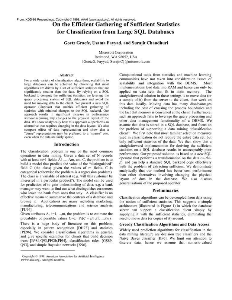
Classification algorithms can be de-coupled from data using
the notion of sufficient statistics. This suggests a simple
architecture (illustrated in Figure 1) in which the database
server can support a classification client simply by
supplying it with the sufficient statistics, eliminating the
need to move data (or copies of it) around.
Greedy Classification Algorithms and Data Access
Widely used prediction algorithms for classification in the
data mining literature are decision tree classifiers and the
Naïve Bayes classifier [K96]. We limit our attention to
discrete data, hence we assume that numeric-valued
SQL RDBMS
(Extended)
Queries for
counts
Sufficient
Statistics
Produced
Model
Data Mining
Client
Figure 1. Database server and data mining client
attributes have undergone some discretization stage [B*84,
Q93, FI92a, FI93, DKS95, MAR96]. Decision trees are
good at dealing with data sets having many dimensions
(common in data mining applications), unlike other
approaches for classification such as the nearest neighbor
[DH73], neural networks, regression-based statistical
techniques [PE96], and density estimation-based methods.
Decision trees can also be examined and understood by
humans, particularly the leaves viewed as rules [Q93].
Algorithms reported in the literature generate the tree topdown in a greedy fashion. A partition is selected which
splits the data into two or more subsets. There are several
partition selection measures. Most are based on preferring a
partition which results in locally minimizing the class
impurity of each subset in the partition [B*84]. Several
measures of impurity exist (e.g. Entropy [Q93], the Gini
Index [B*84]). Other measures outside the impurity family
have also been used: the Twoing Rule [B*84], Gain ratio
[Q86,Q93], the J-measure [GS89] and class orthogonality
[FI92b]. The scheme proposed in this paper can support all
of the above measures.
Sufficient Statistics for Selection Measures
A key insight is that the data is not needed if sufficient
statistics are available. We only need a set of counts for the
number of co-occurrences of each attribute value with each
class variable. Since in classification the number of attribute
values is not large (in the hundreds) the size of the counts
table is fairly small. Continuous-valued attributes are
discretized into a set of intervals. All splitting criteria can be
estimated in a straightforward fashion if one had a table,
which we call the correlation counts table giving the set of
counts of co-occurrences of each attribute with each class:
Table 1: Sufficient Statistics for Classification (CC)
Attribute ID
Attribute Value
Class Value
Count
Table1 (henceforth called CC table) has many uses. Once
obtained, there is no further need to refer to the data again.
In a decision tree algorithm, the single operation that needs
to reference the data are is the construction of CC table. We
restrict our attention to the common case where the number
of values makes the CC table size negligible compared to
the size of the data. This results is a significant reduction in
data movement from server to client.
Consider measures used by algorithms for constructing
classifiers. Impurity measures, e.g. class entropy measure
rely on the probability of any class value Ck in set S:
Pr(C=Ck|S), and measure class impurity of a set S as:
Entropy(S) =
l
−∑ Pr(C = Ck | S ) log(Pr(C = Ck | S )) . Let
k =1
Sj be the subset of S consisting of all data items satisfying
Ai=Vij. The class information entropy of a partition induced
by attribute Ai is defined as: Entropy(S|Ai)=
r1
∑ Pr(Ai = Vij) Entropy(Sj) . ID3, C4.5 [Q93] and CART
j =1
[B*84] select the attribute that minimizes this measure.
The probabilities are estimated by the frequencies of
occurrence of each event in the data subset S. Consider the
table CC (Table 2), and let CC[i, j, k] denote the count of
class Ck when Ai=Vj in S, for j=1,…, ri. Let
l
Sum(i, j) =
∑ CC (i, j, k ) , then Entropy(S|Ai) is given by:
k =1
−
l
Sum(i, j) 
CC[i, j , k ]  CC[i, j , k ]  
 . We can
log
N  k =1 Sum(i, j)
 Sum(i, j)  
j =1
r1
∑
∑
equally well score a partition on a single value versus all
other values (binary split) or other splits involving a subset
of the attributes [F94]. Likewise, many other impurity and
statistical measures can be computed strictly from the values
in the correlation counts table CC. The same holds true for
other measures such as Twoing [B*84] and Orthogonality
[FI92]. Variants such as Gain Ratio [Q93] are obtained by
dividing the above entropy by the entropy of the values of
an attribute (without regard to class); i.e. using the terms
Sum(i, j) above. It should be obvious to the reader how
Gini Index measure in CART [B*84] is derived from CC.
Many other measures of interest in statistics are a function
of only the entries of the CC table. For example, a popular
and simple model is known the Naïve Bayes classifier. If
one were to assume that all the attributes in the data are
conditionally independent given the class, then one can
reliably estimate the probability of the class variable using a
simple application of Bayes rule: Pr(C=Ck|A1,…,Am) =
Pr(C = Ck)
Pr(A1 = V1, ,...,Am = Vm)
m
∏Pr(Ai = Vi | C = Ck) ,
The term
i=1
in the denominator is obtained by summing the terms:
m
k
∑
Pr(C = Ck )
i =1
∏ Pr ob( Ai = Vi | C = Ck ) . The CC table
i =1
again provides needed terms: Pr(Ai=Vj|C=Ck) = CC[i, j, k];
Pr(C = Ck) =
ri
∑ CC (i, j, k ) .
j =1
Sufficient Statistics from SQL Backend
Problem with the Obvious Approach
The first natural question to ask is how to generate the
sufficient statistics using standard SQL? Assuming the data
reside in the table DT with m+1 columns (A1,
A2,…,Am,class), CC (Table 1) for a subset of the data
satisfying condition “Condition”, via SQL code is:
Select “A1” as attrID, A1 as attrValue, class, count(*)
From DT Where condition Group By class, attrID, AttrValue
UNION ALL
Select “A2” as attrID, A2 as attrValue, class, count(*)
From DT Where condition Group By class, attrID, attrValue
UNION ALL
...
Select “Am” as attrID, Am as attrValue, class, count(*)
From DT Where condition Group By class, attrID, attrValue
The UNION is needed to obtain counts for each of the
attributes A1,…,Am with the class. We introduce the
condition some_condition to obtain the counts for subsets of
the data (e.g. individual nodes in a decision tree, etc.)
Most database systems will implement such UNION queries
by doing a separate scan for each clause in the union since
the optimizers will be unable to harness the commonality
among the UNION queries. Observe that the form of the
SQL statement using UNION is different from the CUBE
operation proposed in [GC*97]. Unlike CUBE, the grouping
columns only share the class attribute and no grouping is
required for combinations of other attributes. Since we
intend to perform such queries over large tables with many
columns (hundreds), m scans become quite expensive, we
consider methods for avoiding the multiple scans.
New Approach: Unpivoting the Table DT
To avoid the multiple scans caused by the unions, a simple
solution could be to change the physical layout of the table.
Consider the table DT and suppose each row in DT (each
case) were represented as a set of rows, one for each
attribute-value pair. We call this table an “unpivoted” form
of the table and illstrate it in Table 2:
Table 2: Unpivoted form of DT: UDT
Case ID
Attribute ID Attribute Value Class
Why would the UDT form appear to be preferable over DT
form for constructing the CC table in SQL? The answer is
simple. The query to construct CC, consisting of the union
of m sub-queries shown above, reduces to the following
simple query over UDT:
Select AttributeID, AttributeValue, class, count(*) From UDT
Where condition Group By class, AttributeID, AttributeValue
The reader will note that this query will cause only one scan
the table UDT. This is a big win over the m scans required
for DT. However, we show next that this win comes at a
surprisingly steep increase in the cost of the data scan.
Problem with Materializing Unpivoted Table UDT
Consider the scan cost of each of DT and UDT. Let N
denote number of cases, m the number of attributes. We
assume the cost of storing an attribute value is a constant v
bytes. We assume each attribute Ai has value density
d i ≤ 1.0 , i.e. that on average, the proportion of cases over
which the Ai has non-NULL value is di. We assume that the
caseID requires log(N) bits to represent (a lower bound).
Similarly, for m attributes, log(m) bits are needed to
identify an attribute (a lower bound).
Cost of Scannig DT is: N ⋅ m ⋅ v since every attribute value
occupies space in DT. Cost of scanning UDT is:
m
N(
∑ d (log N + log m + v)) . Difference in scan costs is:
i
i =1

∆ = N



m
∑ d i (log(Nm) + v) − mv  . Assuming same density,

i =1
m
then ∀i, di=d, hence ∑ d i = md , yields the simplified form
i =1
of
∆/N= ∑ d i (log( Nm) + v) − mv = m[d log( Nm) + v(d − 1)]
m
i =1
(cost per case). We now compare the scan costs of DT and
UDT for both dense and sparse data. As we demonstrate
below, even for relatively sparse data, the UDT
representation incurs a high overhead.
Analysis for Dense Data
∆
= m log(Nm) which
When the data is fully dense (d = 1),
N
is consistent with our intuition that the DT representation
6
wins by quite a bit. For typical values of N=10 , m=100,
one can see that for a fully dense data set, scanning the UDT
table costs over 2000 times more (recall log is base 2) than
scanning the corresponding DT table. So for fully dense
table, the unpivoted form UDT is not acceptable.
Analysis for Sparse Data
Let us examine the question of when for a classification
problem, does it make sense to use the unpivoted
representation of UDT over DT. We restrict our attention on
the case of a uniform density d (for all i, di=d). Examining
∆
= m[d log( Nm) − v(1 − d )] yields that the
the form
N
unpivoted representation will only start to win when the
expression goes negative. Hence, recalling that d ≤ 1 , UDT
wins when d log( Nm) < v(1 − d ) , which would require that
v
. Note that for large databases this will
d<
log( Nm) + v
only occur when the data is at fairly extreme values of
densities (for classification, having d=0.5 is considered
quite extreme). Thus, the UDT representation may not be
suitable, even if the data are fairly sparse.
Examples
Realistic settings for: size of case ID 3 bytes instead of
log(N), and size of attr. ID: 2 bytes, and letting v = 2 bytes,
∆
= m[d log( Nm) − v(1 − d )] = 2m(3d − 1)
gives cost /case:
N
6
1: Assume N=10 , 300 attributes (m=300), and that half the
values of all attributes are missing, i.e. d=0.5, then the
difference in scan cost per case is 600(1.5 – 1) = 300.
Hence scanning UDT table is equivalent to scanning an
extra 300 Megabytes of data! Note that this cost grows
linearly with added dimensions and size of original table.
2: For Example 1, assume d=0.9 (a realistic assumption in
typical classification settings) then the difference in scan
cost is equivalent to scanning and extra Gigabyte of data.
Clearly if data is at an extreme of sparseness, then
representation UDT will win, however, such data will not
likely be useful for classification algorithms we consider.
This leaves us with the conclusion that a traditional SQL
backend will not support our gathering of counts efficiently.
We show that with a simple extension to the DBMS engine,
we achieve the best of both data representations, enabling a
traditional engine to service these counts efficiently while
operating over the table DT.
The Unpivot Operator
Our key insight is that we can realize the advantage of the
UDT representation without paying the overhead of data
scans if we generate the unpivoted view of the data on-thefly during query processing. We propose a simple extension
to SQL that will enable us to gather the desired sufficient
statistics from DT while avoiding extra data scans. We
introduce operator UNPIVOT, which gives us the desired
unpivoted view of the data, without changing the efficient
DT representation of the data on disk. The proposed
UNPIVOT operator consumes each row of the table DT and
produces m rows. Essentially it performs the translation
from DT representation to UDT representation row by row.
We propose the following syntax for the operator that would
transform the table DT to the table UDT
DT.UNPIVOT(Attr_val for AttrID in (A1,..,Am)).:e need not
transform the stored table, since as was shown above, we do
not want to scan the unpivoted table. Armed with the
UNPIVOT operator, we can now extract the set of sufficient
statistics CC from table DT using the following SQL query:
Select AttrID Attr_val, Class, count(*)
From DT.UNPIVOT(Attr_val for AttrID in (Attr_1,..,Attr_m))
Group by AttrID, Attr_Val, Class
Essentially the DT.Unpivot() operator generates a view of
DT that is equivalent to UDT (Table 2). This view can be
computed and consumed efficiently in a pipeline of
operations and will not be materialized. Hence the penalty
in scan performance illustrated by the analysis will not be
incurred. We achieve a guarantee of a single scan execution
and utilization of the standard DBMS engine support to
derive the desired counts table CC (Table 1).
Incorporating Unpivot operator in Relational Systems
The Unpivot operator, as conceived for data mining and
classification applications, is designed to be integrated into
relational algebra. It consumes a table, such as DT, and it
produces a table, such as UDT. Thus, relational algebra
remains closed even after this addition. The proposed syntax
is a logical and compatible extension of previous algebraic
extensions of the SQL language standard, e.g., the outer join
operations in SQL: “select * from departments d left outer
join employees e on d.dept-id = e.dept-id”. In other words,
there is a well-established precedent for extending the SQL
language with relational algebra operations in the “from”
clause.
As an algebraic operator, Unpivot can be applied to any
intermediate result. For example, in order to apply a search
predicate to a table prior to applying the Unpivot operation:
Select AttrID Attr_val, Class, count(*) From (Select * From
DT Where some-condition).UNPIVOT(Attr_val for AttrID in
(Attr_1,..,Attr_m)) Group by AttrID, Attr_Val, Class
The key to this flexibility is the fact that relational algebra is
closed and therefore permits free composition.
Efficiency of execution for queries employing the Unpivot
operation must be considered. Input rows can be processed
one at a time, and the required processing is a mere copying
of row values; thus, the implementation code for the
Unpivot operator is simple and very fast. Moreover, since
one row’s output is completely independent of any other
row’s, parallel execution can easily be achieved by
partitioning the input rows. In a modern, extensible database
query execution engine based on uniform algorithm
interfaces [G93], adding a new algorithm relatively easy.
Finally, an Unpivot operation affects optimization of neither
the query feeding the Unpivot operator’s data stream nor
that of the query consuming the Unpivot operation’s output
data stream. Thus, index selection based on selectivity and
cost estimates are not hampered by the Unpivot operator. In
a modern database query optimizer based on algebraic
rewrites (e.g. [H89, G95]), the Unpivot operation can be
deeply integrated into the query optimizer, and rewrites can
be defined that move selection predicates and other
operations “up” and “down through” the Unpivot operation.
Hence, Unpivot can be integrated into query optimization
process as deeply as relational selection and joins are today.
Staggered Applications of UNPIVOT operator
We show how the applications of multiple (two) unpivot
operators may be composed for more complex cases of
classification when there are either multiple class columns
or “attribute” and class columns overlap.
Multiple Class Columns
There could be multiple columns that are to be treated as the
“class” columns for CC purposes. If DT had M class
columns: (CaseID,A1,A2,…,Am,Class1,…, ClassM), then:
DT.Unpivot(Attr_val for AttrID in (Attr_1,..,Attr_m) )
will produce a table with 3+M columns (when M=1 we had
4 resulting columns). Now, we will need to execute a union
of M group by operations on the resulting unpivoted table to
obtain our desired counts against each of the Class1,…,
ClassM columns. However, a clever second application of
UNPIVOT will in fact remove the need for the multiple
Group By’s. The second UNPIVOT on the output of the
first UNPIVOT reduces it down to a table of 5 columns,
then a single Group By achieves the desired CC table:
Select AttrID, Attr_val, ClassID, ClassVal, count(*) From
DT.UNPIVOT(Attr_val
for
AttrID
in
(A1,...,Am)
).UNPIVOT(ClassVal for ClassID in (Class1,...,ClassM) )
Group by AttrID, Attr_Val, ClassID, ClassVal
Overlapping “Attributes” and “Class” Columns
The “class” and “attribute” columns may not be mutually
exclusive. In general, we would like to treat I of the M
columns as “class” columns. For any particular set of counts
with respect to any fixed “class column”, say column j, we
would like to treat all other M-1 columns as “attributes”.
Let DT consists of the following M columns: (A1, A2, … ,
AM). Assume A1 and A2 are “class” variables, that is, we
would like to see the number of times the value of attribute
A1 co-occurred with the values of every attribute in
A2,…,AM. Same for A2. A simple solution is to preprocess
the table DT and replicate the “class” columns as additional
columns on a new table DT2 which will now have M+2
columns, then carry out the steps above. However, consider
this usage of UNPIVOT :
Select AttrID, Attr_val, ClassID, ClassVal, count(*) From
( Select * from (Select A1,…,Am, A1 AS Class1, A2 AS
Class2 from DT).UNPIVOT(Attr_val for AttrID in
(A1,...,Am) ).UNPIVOT(ClassVal for ClassID in (Class1,
Class2) ) Group by AttrID, Attr_Val, ClassID, ClassVal
This produces the output table of Extension 1 above as
desired. Note that column replication of A1 and A2 was
achieved by the (Select A1,…,AM, A1 AS Class1, A2 AS
Class2 from Data_table) statement embedded in the query.
There is a potential added scan cost due to column
replication, but since the replication is embedded in a
pipeline, we assume the table with replicated columns will
not be materialized. If replication can be done in the
pipeline as an intermediate step, then the technique can be
employed to achieve the desired effect efficiently.
Related Work
With proposed extension using Unpivot and architecture of
Figure 1, performing classification is reduced to using a
simple data mining client that repeatedly queries the
database. For decision trees, all the client needs to do is
maintain the decision tree structure and implement the
scoring functions to be used in selecting the partition at any
node in the decision tree. The basic function of the client is
to issue a series of queries for requests for counts tables for
the nodes in the decision tree being constructed. Interface
with the server is straightforward SQL (with our extension).
Naïve Bayes is even simpler requiring only one scan.
There is a fairly extensive literature on decision tree
generation. Since the implementations available for these
communities assume the data to be in memory, much of the
work has been with very small data sets, typically in the
hundreds to thousands of records. Some authors have
outlined the challenges of dealing with large data stores
[J97]. Much of the work is still focused on virtual memory
systems or in-memory caches [ML98].
More recently, data mining and database research has
addressed the problem of scaling classification algorithms
[J97, MAR96]. The notion of collecting sufficient statistics
has been advocated by [J97], but without consideration of
issues of integration within the database server. The
algorithms in [MAR96] copy the given data set into data
structures that correspond to vertical partitions of the table
(one partition for each attribute), with at least the class
attribute replicated. For high dimensional data, such
replication results in increased scan cost. In contrast, we
avoid the need to create vertical partitions. An alternative
perspective on the Unpivot operator is that it computes all
such vertical partitions on the fly by virtue of data
transformation in an execution pipeline without
materializing the new data view in a single scan over the
data table. We also provide a natural, and fairly minimal,
extension to SQL. Hence, most of the SQL backend need
not be affected. The fact that our scheme does not require
copies of the data table such as vertical partitioning makes
our approach easier from the point of view of data
administration as well.
References
[B*84] L. Breiman, J.H. Friedman, R.A. Olshen, and C.J. Stone, 1984.
Classification and Regression Trees. Monterey, CA: Wadsworth &
Brooks.
[DKS95] J. Dougherty, R. Kohavi, and M. Sahami, 1995. “Supervised and
unsupervised discretization of continuous features.” Proc. of 13th Int.
Conf. On Machine Learning, pp. 194-202. Morgan Kaufmann.
[DH73] R.O. Duda and P.E. Hart 1973. Pattern Classification and Scene
Analysis. New York: John Wiley and Sons.
[FI93] Fayyad, U.M. and Irani, K.B. 1993. Multi-Interval Discretization of
Continuous-Valued attributes for Classification Learning. In Proc. of the
Thirteenth Inter. Joint Conf. on Artificial Intelligence, Chambery,
France.
[FI92a] Fayyad, U. and Irani K, 1992. "On the handling of continuousvalued attribute in decision tree generation", Machine Learning, 8:1.
[FI92b] Fayyad, U.M. and Irani, K.B. 1992. “The Attribute Selection
Problem in Decision Tree Generation.” In Proc. of the Tenth National
Conference on Artificial Intelligence AAAI-92, pp. 104-110, Cambridge,
MA: MIT Press.
[F94] Fayyad, U.M. 1994. Branching on Attribute Values in Decision Tree
Generation. Proc. 12th National Conference on Artificial Intelligence, p.
601--606, MIT Press.
[FU96] U. Fayyad, R. Uthurusamy (Eds), Communications of ACM
39(11), special issue on Data Mining, 1996.
[G93] G. Graefe: Query Evaluation Techniques for Large Databases.
Computing Surveys 25 (2): 73-170 (1993).
[G95] G. Graefe: The Cascades Framework for Query Optimization. Data
Engineering Bulletin 18 (3): 19-29 (1995).
[GS89] R. M. Goodman and P.J. Smyth, 1989. “The induction of
probabilistic rule sets”, Proc. of 6th Int. Conf. On Machine Learning, pp.
129132. Morgan Kaufmann.
[GC*97] J. Gray, S. Chaudhuri, A. Bosworth, A. Layman, D. Reichart, M.
Venkatrao, F. Pellow, and H. Pirahesh, 1997. “Data Cube: A Relational
Aggregation Operator Generalizing Group-by, Cross-Tab, and Sub
Totals”, Data Mining and Knowledge Discovery, vol. 1, no. 1, 1997.
[H89] L. M. Haas, J. C. Freytag, G. M. Lohman, H, Pirahesh: Extensible
Query Processing in Starburst. SIGMOD Conference 1989: 377-388.
[J97] G.H. John, 1997. Enhancements to the Data Mining Process, Ph.D.
Dissertation, Dept. of Computer Science, Stanford University.
[K96] R. Kohavi, 1996. “Scaling Up the Accuracy of Naive-Bayes
Classifiers: a Decision-Tree Hybrid.” Proceedings of the Second
International Conference on Knowledge Discovery and Data Mining.
AAAI Press.
[MAR96] M. Mehta, R. Agrawal, and J. Rissanen, 1996. “SLIQ: a fast
scalable classifier for data mining”, Proceedings of EDBT-96, Springer
Verlag, 1996.
[ML98] A.W. Moore and M. S. Lee, “Cached Sufficient Statistics for
Efficient Machine Learning with Large Datasets,” Journal of Artificial
Intelligence Research, 1998.
[PE96] D. Pregibon, J. Elder, 1996. “A statistical perspective on knowledge
discovery in databases”, in Advances in Knowledge Discovery and Data
Mining, Fayyad et al ( Eds.), pp. 83-116. MIT Press.
[Q93] J.R. Quinlan, 1993. C4.5: Programs for Machine Learning, Morgan
Kaufman, 1993.