From: ISMB-00 Proceedings. Copyright © 2000, AAAI (www.aaai.org). All rights reserved.
Robust Parametric and Semi-parametric Spot Fitting for
Spot Array Images
Norbert Brändle1 , Horng-Yang Chen1 , Horst Bischof 1 , Hilmar Lapp2
1
Vienna University of Technology
Pattern Recognition and Image Processing Group
Treitlstr. 3/1832, A-1040 Vienna
Tel. +43 1 58801-18360, Fax +43 1 58801-18392
nob@prip.tuwien.ac.at
2
Novartis Research Institute Vienna
Genetics
Brunner Str. 59, A-1230 Vienna
Tel. +43 1 86634-631
hilmar.lapp@pharma.novartis.com
Abstract
In this paper we address the problem of reliably fitting parametric and semi-parametric models to spots in
high density spot array images obtained in gene expression experiments. The goal is to measure the amount
of label bound to an array element. A lot of spots can
be modelled accurately by a Gaussian shape. In order
to deal with highly overlapping spots we use robust Mestimators. When the parametric method fails (which
can be detected automatically) we use a novel, robust
semi-parametric method which can handle spots of different shapes accurately. The introduced techniques
are evaluated experimentally.
Keywords: spot arrays, image analysis, robust methods, parametric fitting
Introduction
Genetic spot array images have to be analyzed in the
course of high-throughput hybridization experiments,
where a spot in the array can identify specific expressed
gene products. Common to all array-based approaches
is the necessity to analyze digital images of the array.
The ultimate image analysis goal is to automatically
assign a quantity to every array element giving information about the hybridization signal (spot fitting or
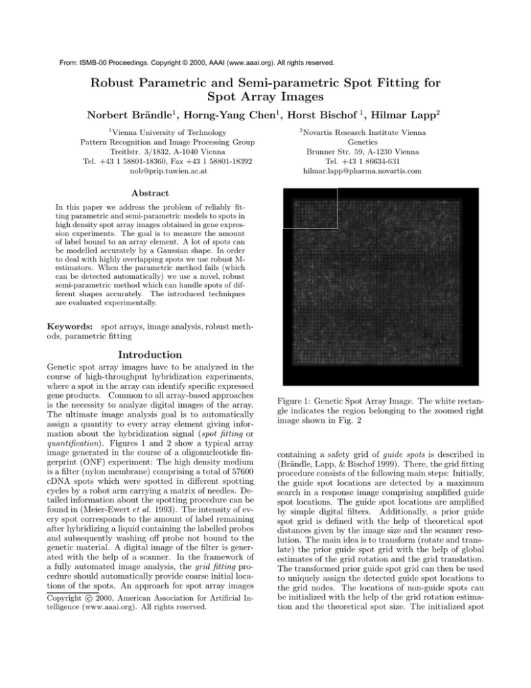
quantification). Figures 1 and 2 show a typical array
image generated in the course of a oligonucleotide fingerprint (ONF) experiment: The high density medium
is a filter (nylon membrane) comprising a total of 57600
cDNA spots which were spotted in different spotting
cycles by a robot arm carrying a matrix of needles. Detailed information about the spotting procedure can be
found in (Meier-Ewert et al. 1993). The intensity of every spot corresponds to the amount of label remaining
after hybridizing a liquid containing the labelled probes
and subsequently washing off probe not bound to the
genetic material. A digital image of the filter is generated with the help of a scanner. In the framework of
a fully automated image analysis, the grid fitting procedure should automatically provide coarse initial locations of the spots. An approach for spot array images
c 2000, American Association for Artificial InCopyright telligence (www.aaai.org). All rights reserved.
Figure 1: Genetic Spot Array Image. The white rectangle indicates the region belonging to the zoomed right
image shown in Fig. 2
containing a safety grid of guide spots is described in
(Brändle, Lapp, & Bischof 1999). There, the grid fitting
procedure consists of the following main steps: Initially,
the guide spot locations are detected by a maximum
search in a response image comprising amplified guide
spot locations. The guide spot locations are amplified
by simple digital filters. Additionally, a prior guide
spot grid is defined with the help of theoretical spot
distances given by the image size and the scanner resolution. The main idea is to transform (rotate and translate) the prior guide spot grid with the help of global
estimates of the grid rotation and the grid translation.
The transformed prior guide spot grid can then be used
to uniquely assign the detected guide spot locations to
the grid nodes. The locations of non-guide spots can
be initialized with the help of the grid rotation estimation and the theoretical spot size. The initialized spot
5500
5000
50
3. Various spot shapes: Depending on the type of the
experiment different spot shapes are possible (Fig. 4).
4500
4000
100
3500
3000
2500
150
2000
1500
200
1000
Figure 4: Spots with uncommon shapes
500
250
50
100
150
200
250
300
350
Figure 2: Genetic Spot Array Image. Zoomed image
corresponding to the white rectangle of Fig. 1
locations are refined by the methods described in this
paper. We first describe the main problems of quantification and the problem of background estimation. The
next section deals with non-robust and robust parametric spot fitting. Then we introduce a semi-parametric
spot fitting method. Finally, we present experimental
results on real data.
Quantification
The goal of the spot fitting procedure is to provide an
accurate estimate of the volume, i.e. the amount of
genetic material of every spot. It must cope with the
following three major problems:
(a) Artifacts
(b) Overlapping spots
Figure 3: Spot fitting problems
1. Noise and outliers: Sometimes gross errors like artifacts which do not comprise gene expression information can occur (Fig. 3a).
2. Overlapping spots: Spots with high intensity or spots
in low-resolution images may interfere with neighboring spots (Fig. 3b).
We decided to use parametric spot models, i.e. twodimensional analytic models the parameters of which
are fitted to the given spot data. This allows us to
deal adequately with the phenomenon of overlapping
spots. However, parametric spot models rely on a priori assumptions about the spot shape which cannot always be guaranteed. We therefore also introduce a more
flexible semi-parametric spot fitting procedure. Noordmans and Smeulders (Noordmans & Smeulders 1998)
provided a general approach for the detection and characterization of overlapping spots. However, their approach is restricted to parametric models and is nonrobust. Robustness is required in order to deal with artifacts. In the following two sections we describe both
a parametric and a non-parametric approach for spot
fitting.
Estimating the Background
A problem independent of the spot fitting strategy is
the fact that the background values (areas with no hybridization signal) need not be uniform across the spot
image. The background values are an important additive constant for spot models. In order to obtain continuously varying background values for the entire image we estimate the background in a global manner.
In principle, the background image is the spot image
subtracted by the quantified spots. However, the information about the hybridization signal is available after
the spot fitting. To tackle this chicken-egg problem, we
estimate the background in two passes. The method
we show is applicable to spot arrays with a small percentage of hybridized spots including a guide spot safety
grid, like the ONF image in Fig. 1. An adaption to other
kinds of spot array images is straightforward. The grid
fitting procedure provides us with the locations of the
guide spots. We furthermore know that the guide spots
always have a (strong) hybridization signal. As a first
approximation we could therefore subtract the pixels
belonging to the guide spots from the spot image. In
order to get smooth results, we use a hierarchical interpolation method based on Gaussian image pyramids
(Jolion & Rosenfeld 1994). An image pyramid combines
the advantages of high and low resolution. It is a collection of images S[l] of a single scene at exponentially
S [l top ]
S [l max ]
SUBTRACT
REDUCE
G[l top ]
G[l max ]
REDUCE
G[ lmax 1 ]
S [l max 1 ]
REDUCE
REDUCE
S [l max 2 ]
G[l max 2 ]
B[l max ]
B[l max 1 ]
EXPAND
S [l ] : Spot Image Pyramid
EXPAND
B[l ] : Background Image Pyramid
B[l max 2 ]
G[l ] : Synthetic Guide Spot Image
(Pass 1)
: Synthetic Spot Image
(Pass 2)
Figure 5: Principle of Background Estimation
decreasing resolutions l ∈ {0 . . . ltop }. The bottom level
of the pyramid is the original image. In the simplest
case, each successive level of the pyramid is obtained
from the previous level by a filtering operation followed
by a sampling operator (Haralick, , & Shapiro 1991).
Figure 5 plots the principle of the background estimation with image pyramids.
Pass 1 This pass is performed after grid fitting and
before the spot fitting. A pyramid S[l] of the spot image
and a pyramid G[l] of the synthetic guide spot image
are built. At the level lmax the resolution of the images
is so low such that the guide spot grid structure is no
longer present in the images, meaning that the guide
spots are merged. At the merging level lmax we subtract G[lmax ] from S[lmax ] resulting in a low-resolution
background image B[lmax ] . In order to get a background
image at the original resolution of the spot image, the
levels of the background pyramid are computed by the
EXPAND function, which consists of bicubic interpolation of the grey values (Press et al. 1992).
Pass 2 The background is estimated a second time
after the spot fitting procedure has finished. With the
knowledge about the model parameters for every spot
we are able to reconstruct a complete synthetic spot
image (see also Fig. 15). The pyramid G[lmax ] in Fig. 5
is now the reconstructed synthetic spot image. The
subtraction and the expansion are performed the same
way as in pass 1.
Parametric Spot Fitting
A parametric fit on a set of intensities (pixels) belonging
to a spot assumes a given analytic model the unknown
parameters of which have to be determined. The ap-
proximate initial locations of the spots are given by the
grid fitting procedure. The extension of the pixel set
belonging to a spot is determined by the prior knowledge about the theoretical spot size, which in return is
given by the image size and the scanner resolution. In
this section we first introduce a Gaussian spot model.
We then describe a non-robust fit for the Gaussian parameters. In the last part of this section we introduce
a robust spot fitting method.
The Gaussian Spot Model
Let S = {(pi , zi ), p ∈ R2 , zi ∈ R} be a set of n points
corresponding to a spot, where zi denotes the intensity at location pi . An initial analysis has shown that
most of the spots can be characterized fairly accurately
by a Gaussian shape. The (non-normalized) Gaussian
function is denoted as
1
(1)
G(p, µ, Σ) = exp − (p − µ)0 Σ−1 (p − µ)
2
with µ ∈ R2 and Σ ∈ R2×2 (2 × 2 matrix). Let the
Gaussian spot model be defined as
Z(p) = Z(a, p, µ, Σ, b) := a G(p, µ, Σ) + b
(2)
with the following parameters:
1. a is the amplitude of the Gaussian model corresponding to the “height” of the spot.
2. µ is the mean of the Gaussian model corresponding
to the “center” (location) of the spot.
3. Σ is the 2 × 2 dispersion matrix:
2
σx σxy
Σ=
σxy σy2
(3)
describing the extension of the spot.
4. b is the background value. Note that the background
b(p) is slowly varying over the image. For the characterization of the background of a spot it is sufficient
to take one background sample b(µ) at the spot center µ. Hence we can denote the background simply
as b.
Non-robust Parameter Estimation
The parameters of the Gaussian spot model (2) can be
computed by maximum likelihood (ML) estimators and
minimization of the sum of square errors (Bishop 1995).
Estimating the Mean and Dispersion Matrix
The shape of a spot can be interpreted as a distribution of the x- and y-coordinates. A spot patch
S contains n data points pi and has the intensities
I(pi ). In order to take into account the estimated background value b
b we denote the corrected intensities as
b of the
b, 0) 1 . The ML estimate µ
zi := max(I(pi ) − b
1
since the background can be overestimated – especially
in the first background estimation – we correct negative values to zero
center µ is then computed as follows:
n
1X
b=
zi pi
µ
T i=1
Robust Parameter Estimation
(4)
where T is the total sum of the corrected intensities of
the patch:
T =
n
X
zi .
(5)
i=1
b of the dispersion matrix
Similarly, the ML estimate Σ
Σ is given by
n
X
b = 1
b i − µ)
b T
zi (pi − µ)(p
Σ
T i=1
(6)
b of the center µ is given by the
Hence, the estimate µ
sample average (i.e. the average with respect to the
given data set) of the coordinates weighted by the corb
rected pixel intensities. Similarly, the ML estimate Σ
of the dispersion matrix Σ is given by the sample avb i − µ)
b T weighted
erage of the outer product (pi − µ)(p
by the pixel intensities.
Estimating the amplitude The estimate b
a of the
amplitude a can be computed by a minimization of the
sum of square errors. Let us define the error function
between the data point and the Gaussian function as
n
o2
1 Xn
b
b Σ)
.
(7)
zi − a G(pi , µ,
E=−
2 i=1
The estimate for a is computed by setting the partial
derivative of E with respect to the parameter a to zero:
n
o
∂E X n
b G(pi , µ,
b = 0. (8)
b Σ)
b Σ)
=
zi − a G(pi , µ,
∂a
i=1
The solution to (8) yields the estimator b
a:
, n
n
X
X
b
b 2.
b Σ)
b Σ)
zi G(pi , µ,
G(pi , µ,
b
a=
i=1
We show how parametric models can be fit in a robust
manner. Information about robust statistics can be
found in (Huber 1981) and (Rousseeuw & Leroy 1987).
One quality measure of a robust estimator is the breakdown point. The breakdown point ∗ gives the limit to
which the percentage of outliers can increase which the
estimator still can tolerate. For instance the breakdown
point of the mean is ∗ = 0.0 and the breakdown point
of the median is ∗ = 0.5 We have chosen M-Estimators
for the spot fitting problem. We first introduce the theory of M-estimators for univariate distributions.
M-Estimators M-Estimators (ML type estimators)
of location are based on the idea of replacing the
squared error between the data and the model by
another function ρ of the error. Let x1 , x2 , . . . , xn
be a sequence of identically independently distributed
observations.
The M-estimator of location µ̃ =
µ̃(x1 , x2 , . . . , xn ) is defined as the solution of the minimizing problem
n
X
ρ(xi − µ) → min
(12)
i=1
with respect to µ, where ρ is a function R 7→ R. If ψ
denotes the first derivative of ρ with respect to µ, the
estimator µ̃ is the solution to the equation
n
X
ψ(xi − µ) = 0.
(13)
i=1
Equation (13) can be written equivalently as
n
X
wi (xi − µ) = 0
(14)
i=1
with
wi =
(9)
i=1
Quantification The brightness V of the spot is estimated as the volume under the fitted Gaussian function:
q
b
(10)
Vb = b
a (2π) det(Σ).
A derivation of the Gaussian integral (10) can be found
in (Bishop 1995). Sometimes the scanner is square rooting the intensities during the scanning process. We
therefore provide an estimator for the brightness W of
the spot with squared intensities. Using the fact that
G(pi , µ, Σ)2 = G(pi , µ, 2·Σ), one can easily verify that
q
b
c = (b
(11)
W
a)2 π det(Σ).
The estimators presented so far are non-robust,
meaning that they are sensitive to outliers, like the artifacts in (Fig. 3a).
ψ(xi − µ)
.
xi − µ
(15)
This gives a formal representation of µ as a weighted
mean
, n
n
X
X
wi xi
wi
(16)
µ=
i=1
i=1
with weights depending on the sample. We used the
following ψ-function, known as Tukey’s biweight:
( 2 2
, |x| ≤ a
x 1 − xa
(17)
ψ(x) =
0
, |x| > a
e.g. with a = 4.
Scale invariant M-Estimators The solution to (13)
is not scale-invariant, since in general ψ(cx) 6= cψ(x).
In practice it means that an M-estimator should be supplemented by an estimator of scale. The scale invariant
version of the M-estimator is defined by the solution to
the equation:
n
X
xi − µ
= 0.
(18)
ψ
σ
i=1
This procedure is also called studentizing. Since σ is
usually unknown it is replaced by an estimator of the
scale. A widely used estimator for the scale is the standard deviation, however it is not robust. So a robust
substitute for the scale must be found. Usually one
takes the MAD (median absolute deviation) divided by
0.6745:
median|xi − median(xi )|
.
(19)
σ̃ =
0.6745
The MAD is a robust estimator for u0.75 · σ = 0.6745σ
(u0.75 is the 0.75 quantile of the standard normal distribution ). So MAD/0.6745 is a robust estimator for
σ.) The breakdown point of this estimator is ∗ = 0.5.
The theory of robust M-estimators for multivariate
distributions with elliptically symmetric density function is studied by Maronna (Maronna 1976). We adapt
the approach for location estimates to our needs (overlap and outlier handling) and therefore use a weighting scheme based on the deviation from the Gaussian
model.
Estimating the Mean and Dispersion Matrix
b for the location µ is computed as
The M-estimate µ
, n
n
X
X
b=
w1 (ei )zi pi
w1 (ei )zi
(20)
µ
i=1
i=1
where the weights are defined as
ψ(x)
(21)
w1 (x) =
x
with Tukey’s biweight (17) as the ψ - function and a =
5. The studentized error ei between the data and the
model for each point is
b
b Σ))
a G(pi , µ,
b := (zi − b
b Σ)
a, b
b, µ,
(22)
ei := ei (b
σ
b of the disperwith unknown spread σ. The estimate Σ
sion matrix Σ is given by the weighted outer product
as
n
X
b = 1
b i − µ)
b T
w1 (ei )2 zi (pi − µ)(p
(23)
Σ
T i=1
with T as the total sum of the intensities of the patch
(Eq. 5).
Estimating the Amplitude The M-estimate b
a of
the amplitude a is given by
n
X
b
b Σ)
w1 (ei )zi G(pi , µ,
b
a=
i=1
n
X
.
(24)
b 2
b Σ)
w1 (ei )G(pi , µ,
i=1
with w1 and ei as defined in (21) and (22) respectively.
Computation of the Parameter Estimators In
general, an M-estimator cannot be computed directly.
An iteration scheme has to be used instead. The equab (23)
b (20), the dispersion matrix Σ
tions for the mean µ
and the amplitude b
a (24) can be solved by the weighted
least square iteration:
, n
n
X
X
µj+1 =
w1 (eij )zi pi
w1 (eij )zi
(25)
i=1
i=1
n
X
b j+1 = 1
w1 (eij )2 zi (pi − µj )(pi − µj )T
Σ
T i=1
n
X
aj+1 =
(26)
w1 (eij )zi G(pi , µj , Σj )
i=1
n
X
(27)
w1 (eij )G(pi , µj , Σj )2
i=1
with w1 as defined in (21) and
eij =
(zi − aj G(pi , µj , Σj ))
σj
(28)
and the MAD (19) adapted to the deviation from the
Gaussian model as the estimate for the scale
σj = mediani∈I ∗
|aj G(pi , µj , Σj ) − zi |
,
0.6745
(29)
where I ∗ = {i | G(pi , µj , Σj ) < c}, e.g. c = 1.6 ∗ u0.95
where u0.95 denotes the 0.95 quantile of the standard
normal distribution.
Managing Overlapping Spots
The problem when fitting models to overlapping spots is
that they will be biased towards the overlapping neighbor. This will result in dislocated fitted models and a
too high quantification. One possible method to tackle
this problem is to correct the input intensities for a spot
by subtracting overlapping neighboring models. However, usually too much is subtracted due to the overlapping situation, such that an iteration process between
subtracting neighbor models and re-fit is needed. Another possible approach the usage of robust estimators.
Intensities which are too high due the overlap are regarded as outliers and are subsequently down-weighted.
In our paper we use a combination of the two schemes:
In a first step a robust fit is performed, then the background estimation is improved and finally a robust re-fit
is performed on the data with subtracted neighboring
models.
Subtracting neighboring models Let G be the
grid of spots defined as G = {gij | i ∈ {1, . . . , IG }, j ∈
{1, . . . , JG }}. For each spot gij let us assume we have
computed a spot model Zij (p, q) with the parameter
vector q ∈ Rk and spot location p ∈ R2 . Consider the
image patch Sij = Sij (p) for gij . In order to take into
account overlapping spots we can recompute the model
Zij by using the modified spot patch
X
∗
= Sij −
Zi+k j+l
(30)
Sij
k,l∈{−1,0,1},(k,l)6=(0,0)
i.e. subtracting neighboring spot models. We furthermore set the models Zij := 0 for i ∈ {0, IG + 1} ∨ j ∈
{0, JG + 1} in oder to deal with the special cases of border points. One could iterate this procedure for every
spot gij over the whole image. One then gradually obtains better models for every spot, stopping when the
parameters of the model for each spot stabilize.
Semi-parametric Spot Fitting
A semi-parametric approach can describe the spot
shape more accurately in the case of deviations from
the model assumptions, which is the case in Fig. 4.
However, overlap handling will be difficult, because a
semi parametric fit will lack an intrinsic declension of
the tails of a parametric model.
Algorithm
The basic idea of this method is to reduce dimensionality of given data using prior knowledge. Assuming
that the spot has elliptically symmetric shape the fit is
computed in the following steps:
A. Find the spot center We first perform a Gaussian fit computing M-estimators for µ and Σ as deb is the spot
scribed in (20) and (23). The estimate µ
center. Since the M-estimator of the location is robust it will also deal with spots with uncommon shapes.
Passing a line perpendicular to the x, y-plane through
b gives us the axis a.
µ
B. Transform the points The estimated dispersion
b gives us an ellipse in the x, y-plane. Let
matrix Σ
b (without loss
e1 and e2 be the two eigenvalues of Σ,
of generality e1 ≥ e2 ), v1 and v2 the corresponding eigenvectors and be the half-plane spanned by
λ1a + λ2 v1 ; λ1 ∈ R, λ2 ∈ R+
0 . Consider the one parametric family of ellipses with the principle axis directions v1 and v2 , and diameters λe1 and λe2 , λ ∈ R+
0
and center µ. The family covers the x, y-plane without
intersection, each point in the x, y-plane lies exactly
on one ellipse. We “rotate” the given intensity points
(pi , zi ) following the path corresponding to pi into the
half-plane yielding a point cloud P aramV ector i in 2space (see Fig. 13f. The first coordinate can be easily
computed by:
q
(31)
e1 · |p|2/ e21 (p · v1 )2 + e22 (1 − (p · v1 )2 )
and the second coordinate is the unchanged zcoordinate.
C. Compute a profile We introduce a simplified,
efficient and robust version of curve approximation for
scattered points suited to our purpose. First we compute m points ci = (xi , yi ), i = 1, . . . , m well describing the shape of curve to be computed. Consider the
vertical parallel strip with y-axis and x ≡ max xi as
borders. We then segment the strip into m commensurate parallel strips and compute ci = mediank rki ,
where rki are those points qk lying in the ith strip, see
Fig. 13f. We further cut off tails of the profile by gradually lowering the profile points down to zero in the last
quarter, because 1) especially at the tail there may be
some overlapping situation and 2) generally there are
fewer points at the tail. For our purpose it is enough to
interpolate the points ci by a polygon and to perform a
smoothing scheme on the profile points, e.g. by replacing each point with a weighted sum of its neighbors.
Alternatively one can compute a spline interpolating
the points ci for the profile curve.
D. Compute Volume The profile curve is rotated
following the elliptical paths as in step B. The brightness V of the spot is then estimated by taking
m
e2 1 X 2
·
(x
+ xi−1 xi + x2i )π(yi − yi−1). (32)
Vb =
e1 3 i=2 i−1
In order to yield good results one should use known numerical integration schemes as (composite) Simpson’s
rule.
Relative Error and Goodness-of-Fit
In order to quantitatively assess how well the (Gaussian) model assumption holds for a given set of n intensities zi belonging to a spot we introduce a measure
for the error. We apply an approach also used in linear
regression analysis as in (Hartung 1989) by comparing
the model to a “standard model Z0 ”:
, n
n
1X
1X
2
(zi − Z(pi ))
(zi − z0 )2
(33)
T1 :=
n i=1
n i=1
P
zi as the mean of the given intensity
with z0 := n1
values. The standard model Z0 in this case is a plane
parallel to the image plane at the height z0 , i.e. Z0 ≡ z0 .
T1 relates the mean squared error between the Gaussian
model and the data to the mean squared error between
a constant model and the data. T1 can also be regarded
as the mean squared error between the Gaussian model
and data normalized by the variance of the error. We
will call T1 the relative squared error or for short relative
error. In the literature 1 − T1 is called the goodness-offit.
Spot Detection Limit
A spot fitting algorithm should decide whether a location contains a spot before performing a fit. Imagine
having input intensities with perfect zero values, computing the mean would lead to a division by zero or
leading to a singular dispersion matrix. This can happen rather often since the first background estimation
is overestimating the background.
One could use our test for goodness-of-fit as spot detection by testing the “Zeromodel” Zzero ≡ 0 being
’d-appropriate’ or not, using the test statistic:
n
P
T1 := d2 · P
n
i=1
i=1
Grid Fitting
1st Background
Estimation
For each spot
zi2
(zi − z0
(34)
Spot Detection
)2
e.g. d2 = 2. However, this measure is non-robust. We
use instead
T2 := median(zi ) > d
(35)
for spot detection where d = log(2) · V ∗ /n and V ∗ is
the minimum volume a location carries where a spot
still can be expected. The interpretation is that if the
volume of a location V is greater than V ∗ , we expect
that there is P
a spot. The easiest way to estimate the
volume is n · zi , leading to
X
zi > V ∗ /n.
(36)
T2a :=
Spot?
yes
no
Robust
Gaussian Fit
Zero Model
Last Spot?
2nd Background
Estimation
For each spot
In order to overcome noise and outliers for example due
to overlaps we use the median. Assuming that zi is exponentially distributed which comes close to our situation, the log(2) ≈ 0.6931 times the median estimates
the mean. Replacing the mean by the median yields T2 .
Subtract
Neighbors
Spot Fitting Algorithm Overview
Robust
Gaussian Fit
Fig. 6 shows an overview of the spot fitting algorithm.
After the grid fitting the first pass of the background
estimation takes place. After the background estimation a spot test based on (36) is performed for every
spot location . In case of a hybridized spot the parameters of a Gaussian spot model (2) are fit to the intensity data with M-estimators. After the second pass
of the background estimation the neighborhood models are subtracted in order to cope with overlap. If the
subsequent robust Gaussian fit has a high relative error (33) a semi-parametric fit is performed. Finally, the
volume of the spot model is computed.
Experimental Results
Artifacts
Consider the patch in Fig. 7a. The prior spot locations
after the grid fitting are shown in Fig. 7b. The spot
(3, 3) in the center is distorted by an artifact. As can
be seen in Fig. 8a, a simple Gaussian fit will fail, because the location is biased towards the location of the
artifact. The robust Gaussian fit can overcome the outlier. Figure 8b shows the result after 6 weighted least
squares iterations. The label “vol.” denotes the volume of the spot and “qvol.” denotes the volume with
squared intensities.
Spot?
no
Zero Model
yes
Good Fit?
no
SemiParametric Fit
yes
Compute
Volume
Last Spot?
Figure 6: Spot Fitting Overview
Overlapping Spots
We demonstrate how the robust Gaussian fit works on
image data with overlapping spots. Figure 9a shows a
5×5 block originating from an ONF image with low resolution. Figure 9b shows the prior spot locations after
the grid fitting. Before a fit is performed a spot detection limit as introduced in (35) is computed with limit
V ∗ = 30000 corresponding to d = 400. In Fig. 10a the
white marks indicate the detected spots. Fig. 10b shows
a 3D plot of the block. Almost all locations are classified
correctly including location (5, 1), where a neighboring
spot is interfering from the left. Location (2, 1) is falsly
5000
(1,1)
(1,2)
(1,3)
(1,4)
(1,5)
(2,1)
(2,2)
(2,3)
(2,4)
(2,5)
5000
4500
(1,1)
(1,2)
(1,3)
(1,4)
(1,5)
(2,1)
(2,2)
(2,3)
(2,4)
(2,5)
(3,1)
(3,2)
(3,3)
(3,4)
(3,5)
(4,1)
(4,2)
(4,3)
(4,4)
(4,5)
(5,1)
(5,2)
(5,3)
(5,4)
(5,5)
4500
5
5
4000
4000
3500
10
10
3500
3000
(3,1)
(3,2)
(3,3)
(3,4)
(3,5)
2500
15
5
4000
5
2000
(4,1)
10
(4,2)
(4,3)
(4,4)
2500
3500
2000
(4,5)
3000
15
10
3000
1500
20
2500
15
15
1000
(5,1)
(5,2)
(5,3)
(5,4)
(5,5)
2000
20
1500
1000
2000
1500
20
20
25
1500
500
500
25
1000
25
25
1000
5
10
15
20
5
25
10
15
20
25
5
20
5
25
10
15
20
25
(b) Location Initializations
Figure 9: Block with overlapping spots
Figure 7: Given patch with artifact
Gaussian fit at Location (3,3)
15
(a) Intensities
(b) Prior spot locations
(a) Image data
10
Robust Gaussian fit at Location (3,3)
2000
5000
1500
1000
4500
5
1000
500
0
1
4000
500
3500
10
7
2
6
3
5
4
4
5
3
vol.: 26307.1 6
qvol.: 2.27803e+07
2
7
1
3000
0
1
7
2
15
2500
6
3
4
6 iterations
vol.: 15917.7
qvol.: 9.35413e+06
5
4
5
2000
1500
2
7
1
1000
25
5
(a)
(b)
Figure 8: Dealing with artifacts in Fig.7
detected as a spot, because two neighboring spots are
overlapping. Spot (3,1) is an ordinary spot with no interfering neighbors, the robust estimator stops after 3
iterations without any big changes.
Spots (1, 3), (2, 5) and (3, 3) have up to three overlapping neighbors, here the robust estimator can recover
the original spot location quite well, especially for (1, 3)
and (3, 3). Spot (1, 3) is plotted in Fig. 11a. The nonrobust Gaussian fit is biased towards the neighboring
spots, whereas the location of robustly fitted Gaussian
spot is more plausible. Spots (1, 4), (2, 3) and (2, 4)
have over four overlapping neighbors and are therefore
difficult cases, but still some improvements can be done.
The non-robust and robust Gaussian fits are plotted in
Fig. 11b.
After the first robust Gauss fit we refit on every location with subtracted neighborhood models. The centers
computed during the first fit are taken as the a priori
centers for the second fit. When taking a look at the
new patches with subtracted neighbors (see Fig. 12a)
one will notice that the patches are now less distorted
than the previous patch and are more “spot like” – an
indication that the situation has improved.
When investigating the goodness of fit and the patch
shapes, the first robust fitting resolved the overlaps at
spos (1, 3) (see Fig. 12a) and (3, 3) very well. The re-
3000
2000
1000
0
25
5
20
10
20
3
6
4000
Intensity
1500
Intensity
Intensity
2000
10
15
20
25
500
(a)
15
15
10
20
5
25
(b)
Figure 10: Detected spots and 3D plot of image data
sults for the spots (1,4) and (2,5) are good, the results
for (2,3) (see Fig. 12b) are acceptable, and the results
for (2,4) are not good enough. Generally, on can say
that the robust estimation will perform well up to four
overlapping neighbors while more than four will make
problems. This is can be explained by the fact that
highest possible breakdown point of a robust estimator
is ∗ = 0.5. If more than 50% of the input datas are
false the situation cannot be recovered directly by a robust estimator. An overview of the fitted models can
be seen in Fig. 12c.
Uncommon Shapes
Figures 13a and b show a volcano spot with an overlap from the right hand side. An ordinary Gaussian
fit would be biased to the right neighbor, but a robust
estimator recovers the location easily (Fig. 13c). Performing a robust Gauss fit on both sides we subtract
the neighborhood spot model from the patch receiving
the corrected data (see Fig. 13d). After a Gaussian
refit the initial volume estimation can be observed in
Fig. 13e but the estimated volume is not very reliable
due to the high relative error rate. Using the center
and dispersion we performed a semi parametric fit (see
Fig. 13f). We smoothed the profile points by replac-
Gauss fit at Location (1,3)
Data with Subtr. Neighbors
at Loc. (1,3)
Robust Gauss fit at Location (1,3)
Rob. Gauss
fit at Loc. (1,3)
1000
Intensity
Intensity
Intensity
3000
2000
2000
1000
0
7
2
7
2
5
4
1000
3
2
4
5
7
1
Gauss fit at Location (2,3)
4 iterations
rel.err.: 0.0908397
goodn.: 0.90916
vol.: 40595.6
qvol.: 5.94085e+07
3
6
2
7
1
1
(a) Initial spot fitting for spot (1,3)
5
4
2
7
6
3
4
3
6
7
2
5
4
5
8 iterations
vol.: 46134.6
qvol.: 7.37937e+07
2
1
6
3
5
4
3
6
1000
7
6
4
5
vol.: 54613.7
qvol.: 9.09924e+07
2000
0
1
1
6
3
2000
0
0
1
3000
Intensity
3000
3000
5
3
6
2
7
1
(a) After subtraction of neighborhood models of
spot (1,3)
Robust Gauss fit at Location (2,3)
Data with Subtr. Neighbors
at Loc. (2,3)
Rob. Gauss fit
at Loc. (2,3)
3000
1000
0
2000
3000
1000
0
1
7
2
6
3
5
4
1
7
2
6
3
4
5
vol.: 63847.3
qvol.: 1.02602e+08
3
6
2
7
1
2000
1000
7
2
3
6
1
6
3
2
7
1000
0
1
4
5
2000
0
5
4
15 iterations
vol.: 57870.5
qvol.: 9.52101e+07
3000
Intensity
2000
Intensity
Intensity
3000
Intensity
4
4
1
4
5
2
7
6
3
5
4
3 iterations
rel.err.: 0.178895
goodn.: 0.821105
vol.: 47495.7
qvol.: 6.93349e+07
3
6
7
2
5
1
(b) Initial spot fitting for spot (2,3)
5
We demonstrate the result of the spot fitting for the
image in Fig. 2 containg a total of 40 × 60 = 240 spots.
After the grid fitting we have the prior locations of every
spot and apply the first background estimation routine
to be ready for the first run. A major issue is the detection limit. It determines whether the location possibly
contains a spot of interest. Pretending we do not know
much about the volume of a spot we set V ∗ = 0 using
the detection limit Eqn. 35. The algorithm will then fit
at every location. After a second backgound estimation
and a second run the fits from the first run are refined.
The reconstructed image can be seen in Fig. 15. An
2
7
1
From behind
Gaussian Spots
Entire Image
3
6
(b) After subtraction of neighborhood models of
spot (2,3)
Figure 11: Initial non-robust and robust Gaussian spot
fitting
3000
Intensity
3000
Intensity
ing each point (except at the border) with the weighted
sum over the left, the point itself and right neighbor
with the weights 3,6, and 2. The left neighbor received
higher weights, because the points on the left hand side
are more reliable since they are closer to the center.
The goodness of fit improved and a more reliable quantification is done. We also compared the algorithms to
each other by plotting the percentage of data covered
by the strip with the two offset profile curves as borders yielding a performance curve, see Fig. 14. A quick
ascending curve indicates that the method is performing well, because the data points are covered early. As
one can see the semi-parametric fit is better than the
Gaussian fit.
4
2000
1000
0
2000
1000
0
25
25
25
5
20
20
20
10
15
15
15
15
10
10
10
20
5
25
rel.err.: 0.109603
goodn.: 0.890397
5
5
(c) Models of all detected spots
Figure 12: Detected spots and 3D plot of image data
analysis showed that most of the spots have a volume
between 10000 and 20000 – locations with a volume
lower than 10000 possibly contain no spots. With this
knowledge we set V ∗ to 10000 and rerun our program.
This time no singular locations are detected. In Fig.
16 we plotted the relative error for each spot location.
Some locations have a significant error over 1.0. This
is due to a bad fit as the result of fitting a model to
location containing no spot. A location without a spot
can still pass the detection limit when neighboring spots
are interfering. We therefore perform a post processing
procedure by simply rejecting a model with too high
error, e.g. relative error greater that 0.4. In general,
a relative error smaller than 0.1 indicates a very good,
smaller than 0.2 a good fit, while at values bigger than
100
Vulcano Spot with Overlap
Data Points Included in Percent
90
2000
2500
2
Intensity
1500
4
2000
1000
6
1500
8
500
10
1000
0
12
2
4
500
14
6
8
10
12
16
14
2
4
6
8
10
12
14
16
2
16
(a)
12
10
8
6
4
14
16
(b)
90%−level
80
70
60
50
Gauss fit
Semi param. fit
40
30
20
10
Robust Gaussian fit
Vulcano Spot with Subtracted Neighbor
0
a
2000
0
50
100
150
200
250
300
350
400
Offset
ε
2000
1500
Intensity
Intensity
1500
1000
Figure 14: Semi-parametric fit
1000
500
500
0
0
2
4
6
8
10
12
14
16
7 iterations
4
2
8
6
10
12
14
2
16
4
6
8
10
volume: 73284.5
qvolume: 3.40934e+07
12
14
10
8
6
4
2
16
12
14
16
5500
5000
(c)
(d)
50
4500
4000
Semiparametric fit
100
1200
Robust Gauss fit on Patch with Sub. Neighbor
3500
axis
Gauss
Spline
1000
3000
Linear
2000
Intensity
800
Intensity
1500
1000
4
3
2500
150
5
2
600 1
6
2000
7
500
400
8
0
4
6
8
10
12
rel. error:0.255785
goodness:0.744215
14
16
2
4
8
6
10
12
14
10
16
11
12
0
volume: 88566.9
qvolume: 4.60461e+07
1500
200
9
200
2
0
2
4
6
8
10
rel. error: 0.205373; volume: 80332.2
goodn.: 0.794627; qvolume: 3.90086e+07
13
1000
14
12
500
250
(e)
(f)
50
100
150
200
250
583 spots detected
average rel. error: 0.189113
singular locations: 0
300
350
Figure 13: Volcano Spot with Overlapping Neighbor
Figure 15: Reconstruction of the image in Fig.2
0.4 or 0.5 the fit should be rejected.
Complexity
Table 1 shows the CPU-time costs for each method
per fit in flops (the methods have been implemented
in MatlabTM ). The values should be interpreted as follows:
Resolution →
Method ↓
Gaussian Fit
Semi-param. Fit
Low Res. 7x7
flops/per fit
10.000
2.000
High Res. 16x16
flops/per fit
47.000
15.000
Table 1: CPU-time in Flops
1. A (non robust) Gaussian fit in low resolution requires
approximately 10.000 flops.
2. A robust Gaussian fit with k iterations requires approximately (k + 1) × 10.000 flops (1 fit for the initial
guess and k remaining fits for each iteration).
3. A semi-parametric fit with 5 “profile points” costs
2.000 flops in low resolution, while in high resolution
14 “profile points” are computed requiring 15.000
flops.
4. A single semi-parametric fit is approximately four
times faster than a Gaussian fit in low and high resolution. However, one should keep in mind that a
semi-parametric fit in general can not be performed
directly without any preceding center search by a Mestimator of location.
5. Let n × n be the dimension of the input patch, i.e.
n = 7/n = 16 for low/high resolution. While the
computing time for the Gaussian fit will increase with
O(n2), the computing time for a semi-parametric fit
will increase with O(n2 · log(n)). The reason is that a
Gaussian fit basically sums over all data points while
sorting algorithms are needed for a semi-parametric
fit.
6. An already implemented C-version of the non-robust
3
5
2.5
10
have confidence intervals for the parameters but also
for the volume. Assuming a given center or a perfectly
determined center a confidence interval for the volume
can be directly constructed from a confidence interval
for the amplitude and dispersion matrix.
2
15
20
1.5
25
1
30
0.5
35
40
10
20
30
40
50
60
Figure 16: Relative Error of the 40 × 60 Spots
spot fitting with subtracting neighbors for all spots
needs about four minutes on the same machine (including the grid fitting).
Conclusion
The basic problems in spot fitting are overlapping and
non Gaussian spots. Overlaps with up to three or four
neighbors can be reliably solved by robust fitting and
subtracting neighboring models with a subsequent refit. For overlapping situations with more than four
neighbors too few consistent data is available for robust
estimators. One should remember that the highest possible breakdown point of a robust estimator is ∗ = 0.5.
In such a case one should avoid any fitting and assign a
“standard spot model” to the spot location and do the
first fit after subtracting the neighbors. Such a “standard spot model” can be computed by first estimating
the center by M-estimation of location, second taking
a ’standard’ dispersion matrix (the spots are approximately of equal size) and estimating the amplitude by
least square.
Outlook
We provide the following suggestions for the future
work:
Finding alternative measures for goodness of fit
and detection limit We are rather satisfied with the
introduced measures for goodness of fit and detection
limit. However, one may find an alternative approach
by constructing other statistics or using a (maximum)
entropy method for detection.
Constructing confidence intervals for parameters In statistics it is common to give confidence intervals, ellipses, etc. for the parameters or even for the
model. For our problem it would be useful not only to
Developing machine learning algorithms When
analyzing a ONF-library the computer computes over
4600 million fits. However, the computer does not learn
what is a good fit or what is a spot. It does not learn
that a certain volume estimation cannot be possible.
The computer should adapt to new conditions and be
more fault-tolerant. Robust estimation, detection limit,
fit acceptance depend on parameters the prior choice of
which may not stay optimal from image to image, from
library to library or even from experiment to experiment. Furthermore, the computer could develop some
heuristics like: the Gaussian fit always overestimates
the volume by 10%.
References
Bishop, C. M. 1995. Neural Networks for Pattern
Recognition. Clarendon Press.
Brändle, N.; Lapp, H.; and Bischof, H. 1999. Automatic Grid Fitting for Genetic Spot Array Images
Containing Guide Spots. In 8th Intl. Conf. on Computer Analysis of Images and Patterns, Ljubljana,
Slovenia, September 1–3, 357–366.
Haralick, R. M.; ; and Shapiro, L. G. 1991. Glossary of
computer vision terms. Pattern Recognition 24:69–93.
Hartung, J. 1989. Multivariate Statistik. R. Oldenburg
Verlag München Wien.
Huber, P. J. 1981. Robust Statistics. John Wiley and
Sons.
Jolion, J.-M., and Rosenfeld, A. 1994. A Pyramid
Framework for Early Vision. Kluwer.
Maronna, R. A. 1976. Robust M-estimators of multivariate location and scatter. The Annals of Statistics
4(1):51–67.
Meier-Ewert, S.; Maier, E.; Ahmadi, A. R.; Curtis,
J.; and Lehrach, H. 1993. An automated approach
to generating expressed sequence catalogues. Nature
361:375–376.
Noordmans, H. J., and Smeulders, A. W. M. 1998.
Detection and Characterization of Isolated and Overlapping Spots. Computer Vision and Image Understanding 70(1):23–35.
Press, W. H.; Teukolsky, S. A.; Vetterling, W. T.; and
Flannery, B. P. 1992. Numerical Recipes in C. Cambridge University Press.
Rousseeuw, P. J., and Leroy, A. M. 1987. Robust
Regression & Outlier Detection. John Wiley & Sons.