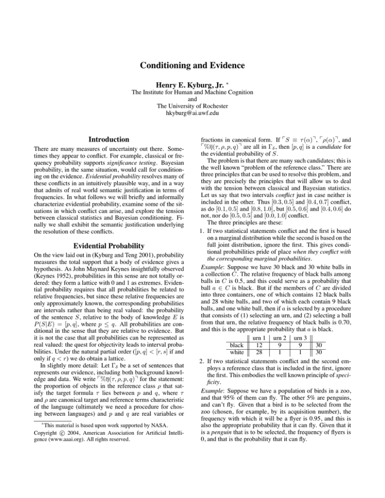
Conditioning and Evidence
Henry E. Kyburg, Jr.
∗
The Institute for Human and Machine Cognition
and
The University of Rochester
hkyburg@ai.uwf.edu
Introduction
There are many measures of uncertainty out there. Sometimes they appear to conflict. For example, classical or frequency probability supports significance testing. Bayesian
probability, in the same situation, would call for conditioning on the evidence. Evidential probability resolves many of
these conflicts in an intuitively plausible way, and in a way
that admits of real world semantic justification in terms of
frequencies. In what follows we will briefly and informally
characterize evidential probability, examine some of the situations in which conflict can arise, and explore the tension
between classical statistics and Bayesian conditioning. Finally we shall exhibit the semantic justification underlying
the resolution of these conflicts.
Evidential Probability
On the view laid out in (Kyburg and Teng 2001), probability
measures the total support that a body of evidence gives a
hypothesis. As John Maynard Keynes insightfully observed
(Keynes 1952), probabilities in this sense are not totally ordered: they form a lattice with 0 and 1 as extremes. Evidential probability requires that all probabilities be related to
relative frequencies, but since these relative frequencies are
only approximately known, the corresponding probabilities
are intervals rather than being real valued: the probability
of the sentence S, relative to the body of knowledge E is
P (S|E) = [p, q], where p ≤ q. All probabilities are conditional in the sense that they are relative to evidence. But
it is not the case that all probabilities can be represented as
real valued: the quest for objectivity leads to interval probabilities. Under the natural partial order ([p, q] < [r, s] if and
only if q < r) we do obtain a lattice.
In slightly more detail: Let Γδ be a set of sentences that
represents our evidence, including both background knowledge and data. We write %η(τ, ρ, p, q) for the statement:
the proportion of objects in the reference class ρ that satisfy the target formula τ lies between p and q, where τ
and ρ are canonical target and reference terms characteristic
of the language (ultimately we need a procedure for chosing between languages) and p and q are real variables or
∗
This material is based upon work supported by NASA.
c 2004, American Association for Artificial IntelliCopyright gence (www.aaai.org). All rights reserved.
fractions in canonical form. If S ≡ τ (α), ρ(α), and
%η(τ, ρ, p, q) are all in Γδ , then [p, q] is a candidate for
the evidential probability of S.
The problem is that there are many such candidates; this is
the well known “problem of the reference class.” There are
three principles that can be used to resolve this problem, and
they are precisely the principles that will allow us to deal
with the tension between classical and Bayesian statistics.
Let us say that two intervals conflict just in case neither is
included in the other. Thus [0.3, 0.5] and [0.4, 0.7] conflict,
as do [0.1, 0.5] and [0.8, 1.0], but [0.5, 0.6] and [0.4, 0.6] do
not, nor do [0.5, 0.5] and [0.0, 1.0] conflict.
The three principles are these:
1. If two statistical statements conflict and the first is based
on a marginal distribution while the second is based on the
full joint distribution, ignore the first. This gives conditional probabilities pride of place when they conflict with
the corresponding marginal probabilities.
Example: Suppose we have 30 black and 30 white balls in
a collection C. The relative frequency of black balls among
balls in C is 0.5, and this could serve as a probability that
ball a ∈ C is black. But if the members of C are divided
into three containers, one of which contains 12 black balls
and 28 white balls, and two of which each contain 9 black
balls, and one white ball, then if a is selected by a procedure
that consists of (1) selecting an urn, and (2) selecting a ball
from that urn, the relative frequency of black balls is 0.70,
and this is the appropriate probability that a is black.
urn 1 urn 2 urn 3
black
12
9
9
30
white
28
1
1
30
2. If two statistical statements conflict and the second employs a reference class that is included in the first, ignore
the first. This embodies the well known principle of specificity.
Example: Suppose we have a population of birds in a zoo,
and that 95% of them can fly. The other 5% are penguins,
and can’t fly. Given that a bird is to be selected from the
zoo (chosen, for example, by its acquisition number), the
frequency with which it will be a flyer is 0.95, and this is
also the appropriate probability that it can fly. Given that it
is a penguin that is to be selected, the frequency of flyers is
0, and that is the probability that it can fly.
3. If a statistical statement that survives (1) and (2) mentions
an interval that includes every interval mentioned by other
survivors of (1) and (2), it may be ignored. We may call
this the principle of relative vacuity.
Example: Suppose we are considering a toss of a coin. The
coin has been extensively tested, and we know that it yields
heads between 0.4 and 0.6 of the time. It is being tossed by
an expert whose record supports the hypothesis that he gets
heads between 0.48 and 0.56 of the time. Of course we also
know that coin tosses in general yield heads very nearly half
the time — say between 0.495 and 0.505 of the time. There
is nothing that conflicts with [0.495,0.505], so the more specific relative frequencies ([0.40,0.60],[0.48,0.56]) can legitimately be ignored.
We obtain a probability interval from these principles by
taking it to be the cover of the conflicting intervals that cannot be ignored on one of these three grounds. In many cases
— for example, those involving well calibrated gambling
apparatus — we can get quite precise probabilities from the
application of these principles. Whether this is always the
case is something we will briefly consider later.
Conditioning
There is no conflict between conditioning and relative frequencies. The classic founding fathers — Neyman, Fisher,
Pearson — all understood Bayes’ theorem to be a theorem,
and took it to be applicable under appropriate conditions —
namely, when there was knowledge of prior distributions.
As Levi (Levi 1980, Chapter 16) showed, there is a conflict between conditioning and direct inference, the foundation of evidential probability. Kyburg has argued against the
universality of conditioning, though direct inference sometims supports it. There is a problem to be faced, but it is
a straight-forward technical one; this is the problem generated by approximate knowledge. Conditional probability
is easy enough to characterize on the basis of point valued
probabilities; but when we must be concerned with intervals or sets of probability functions things are more complicated. Let us observe, first, that most statements of the
form %η(τ, ρ, p, q) are in our bodies of knowledge because they follow from distribution statements that are accepted in our bodies of knowledge. These distribution statements have the form: the random quantity Q has a distribution in R belonging to the nonempty set of distributions D.
If b is a Borel set, we may note that
%x(Q(x) ∈ b, x ∈ R, inf { dD}, sup { dD})
D∈D
b
D∈D
b
has just the form we stipulated for statistical knowledge in
the previous section. As before, Q and R are constrained to
be target and reference terms.
From here to interval-valued conditional probabilities is
a simple hop: condition on each of the underlying distributions for which the conditional distribution is defined.
Example: Suppose our domain is rolls of a die. What
we know of this die is that it is either fair (the distribution corresponds to a frequency function uniform
over the six outcomes) or it is biased in favor of one
and against two, corresponding to a frequency function
3/12, 1/12, 1/6, 1/6, 1/6, 1/6.
The probability of a
five on the next roll is [1/6,1/6] since 1/6 is both the
inf and sup. The probability of a one is [1/6, 3/12].
The conditional probability of a one given an odd outcome on the next roll is obtained from the set of conditional distributions corresponding to the frequency functions
{1/3, 1/3, 1/3, 3/7, 2/7, 2/7} and is [2/6, 3/7].
Significance Testing
Significance testing is one of the most frequently applied
forms of statistical inference. The general pattern is to formulate a hypothesis to be tested, which will be rejected just
in case a particular kind of observation is made. The observation is one that would be very unlikely were that hypothesis to be true. Thus rejecting the hypothesis, when it is true,
will occur rarely.
Example: Suppose we want to test the hypothesis H1
that supplementary vitamin Z improves performance in the
broad jump. Of course we must make this hypothesis more
precise (how much Z? How much improvement? In what
class of people?) But assuming we have done that, the
time honored way of proceeding is to obtain a sample of
that class, to divide them (at random) into an experimental group and a control group, and to test the corresponding
null hypothesis H0 that there is no difference between the
two groups, or rather that any observed difference between
the two groups is due to chance. We reject H0 if we observe
a result in the comparison of the two groups that is too large,
i.e., falls in the rejection region R of our test.
The size of our significance test is the chance of falsely rejecting the null hypothesis; or, given that we have observed
an outcome in the rejection region, it is the chance that the
null hypothesis is true (anyway). If the size of the test is
0.05, and we have observed a point in the rejection region,
the probability of H0 is [0.05,0.05]. Note that if we obtain a
result that is not in the rejection region, we can draw no conclusion at all; this is why Fisher (Fisher 1971) regarded significance testing as only a preliminary of scientific inquiry.
Of course this is assuming no conflict. One way in which
there could be conflict is that the test is a randomized one, in
which an auxiliary experiment determines that the rejection
region is R1 , characterized by a frequency of false rejection
0.014, with probability 0.60, or R2 , characterized by a frequency false rejection of 0.105. In that way we can achieve a
mixture of the two unrandomized experiments with an long
run false rejection rate of 0.05. But both unrandomized experiments conflict with 0.05, and, typically, we will know
the outcome of the auxiliary experiment, and thus the specific rule we followed. Specificity rules out [0.05,0.05] in
favor of one or the other of the more specific alternatives.
Another, more interesting, way in which there could be
conflict is as a result of prior knowledge. If the prior probability of H0 is the whole interval [0,1], then the posterior
probability will cover the same interval, and conditioning
would leave us with the uninformative interval; this is ruled
out by (3). But if the prior probability of the null hypothesis
is not the vacuous interval [0,1], then we may be led to the
conditional probability. When will this be? When the conditional probability conflicts with [.05,0.05], which will be the
case, for a conditional probability [s, t], when t is less than
0.05 or s is more than 0.05.
Let B be our background knowledge, and R be the rejection region, and let
P (H0 |B) = [p, q]
P (R|H0 ∧ B) = [r, r]
P (R|H 0 ∧ B) = [x, y]
P (H0 |R ∧ B) = [s, t]
The lower and upper conditional probabilities are
pr
qr
s=
and t =
pr + (1 − p)y
qr + (1 − q)x
We have a conflict with the significance test just in case
either t is less than 0.05 or s is greater than 0.05. The following table gives a feel for when there is conflict (s > 0.05).
y
0.15
0.25
0.50
0.75
0.95
p 0.136 0.208 0.345 0.441 0.500
Note that whether or not there is conflict depends on the
upper probability of the rejection region given H0 , as well
as the lower probability of H0 . Thus if the probability of
H0 is [0.20,0.40] and the probability of a point in the rejection region, given that H0 is false is [0.10,0.80], then
(since the probability of a point in the rejection region R,
given H0 , is 0.05 by hypothesis) P (H0 |R ∧ B) = [[0.20 ∗
0.05]/[(0.20 ∗ .05) + (0.80) ∗ 0.80)], [0.40 ∗ .05]/[(0.40 ∗
0.05) + (0.60 ∗ 0.10)]] = [0.015, 0.250], which does not
conflict with [0.05,0.05], while the corresponding calculation when the probability, given the denial of H0 , of a point
in the rejection region is [0.10,0.0.20] yields [0.058,0.250],
which does conflict with [0.05,0.05]. Similar considerations
concern the other possibility of conflict.
Hypothesis Testing
In significance testing we are testing a hypothesis H0 against
its denial. In general, the denial of the null hypothesis is not
very informative. In the ideal hypothesis testing case, we
test one hypothesis H0 against a specific alternative, H1 . We
associate such a test, construed as leading to the rejection of
H0 , with two kinds of error: error of the first kind, or type I
error, consists in erroneously rejecting H0 , and error of the
second kind consists in mistakenly failing to reject H0 . The
size of a test, α, is the probability that it will commit an error
of type I. The power of a test, 1 − β, is the probability that it
will avoid committing an error of type II; it is the probability
of obtaining a point in the rejection region under H1 .
The two kinds of error that can be made may both be
bounded. In the case of testing a simple hypothesis against a
simple alternative, both may be quite precise; and this may
provide us with interval bounds on the error of applying a
particular test. If the probability of making an error of the
first kind is α, and the probability of making an error of the
second kind is β, then the probability of making an error
(before conducting the test) is [α, β], assuming α < β.
But of course when we have conducted the test, we know
how the test came out, and so we know whether or not H0
was rejected. If H0 was rejected we know that the probability of error is (in this simple, idealized case) exactly α. If
H0 was not rejected, our error, if any, was that we failed to
reject H0 , even though it was false, i.e., even though H1 was
true, and so the probability of error is β. In either case we
have a precise probability with which to contrast the results
of Bayesian inference.
In general, of course, we are not testing a precise hypothesis against a precise alternative. The hypothesis tested, H0 ,
may be composite. Nevertheless, we can typically find a
value of α that will provide an upper bound for the probability of mistakenly rejecting H0 . The probability of error of
the first kind may thus be the interval [0, α], or the probability of not making an error in rejecting the hypothesis tested
is [1 − α, 1]. Again, typically, we find it even more difficult
to find a lower bound for the power of a test; what is done
is to seek a test of H0 against H1 for which α is bounded
above, and for which the probability of error of the second
kind is minimized among the set of alternatives H1 being
contemplated. (In general H0 and H1 are exclusive, but not
exhaustive.
After the test, this leaves us back in the significance testing state of affairs: if H0 is rejected, we can assign a probability — perhaps the interval [1 − α, 1] — to its denial, but
if H0 is not rejected we are left only with the “conclusion”
that the test in question did not reject H0 ; the probability of
H0 may remain the whole interval [0,1].
The status of Bayesian inference differs sharply in the two
cases, according to whether H0 is rejected or not. When H0
is “rejected at the α level,” the existence of a set of prior
distributions that, conditioned on the same evidence, yields
a posterior probability that conflicts with [1 − α, 1] undermines that rejection, according to the first rule. On the other
hand, when the test fails to reject H0 , the relevant truth frequency of H0 may be the whole interval [0,1], and any (objective) prior distribution that yields a non-vacuous posterior
dominates, according to the third rule.
Confidence Intervals
Inference leading to confidence intervals can be presented as
depending on a lot of background knowledge (for example,
in inferring the length of a table from its measurement we
make use of our knowledge that the distribution of errors of
measurement is Normal), but it is also possible to infer confidence intervals without background knowledge. This case
is particularly interesting as helping to establish the possibility of objective statistical knowledge.
Let B be a finite set of objects; let some of these objects
belong also to C. Let r be the proportion of B’s that are
C. For any value of r, we can easily enough compute upper
U (r) and lower L(r) bounds that constitute the shortest interval into which we can, with a relative frequency of at least
0.95, expect the proportion of C’s in a sample of N B’s to
fall. Of course this depends on r. But this shortest interval
is longest for N/2 or (N + 1)/2. In short, we can know, a
priori, that 95% to 100%of the N -membered samples of B
are representative in the sense that the sample corresponds
to a point between the set of upper U (r) bounds and the
set of lower L(r) bounds. These functions are not continuous — they are step functions — but that need not bother
us since we are dealing in intervals anyway. It did bother
Fisher, who made much of the invertibility of the quantity
— the so-called fiducial quantity — on which the fiducial
inference is based. For this reason he denied the validity of
the method of confidence limits. (Fisher 1956, p.65–66) If f
is the observed relative frequency of C’s in our sample, then
the corresponding bounds on r are given by rl∗ = U −1 (f )
and ru∗ = L−1 (f ) (we adopt the conservative minimum or
maximum if we hit a point of discontinuity).
This proportion can give rise to a probability provided the
three conditions mentioned earlier are satisfied: There is no
interval conflicting with [0.95,1.0] that is based on a distribution of which the distribution just described is a marginalization. There is no subset of the set of N -membered samples that carries a conflicting interval for the conclusion.
And the cover of the set of intervals meeting the first two
requirements is not properly included in [0.95,1.0]. We will
now look at examples of how each of these conditions may
be violated.
Suppose that the population of B’s belongs to a collection
of populations, within which we know something about the
distribution of the proportion of C’s, for example, that the
proportion is itself distributed according to the density function e−x . In this case, of course, we would want to condition
on this prior density in order to obtain a posterior distribution for the proportion of C’s. We calculate the conditional
probability that r ∈ [U −1 (f ), L−1 (f )]. It may conflict with
the interval [0.95,1.0]. If it does, then since the interval
[0.95,1.0] is derived from the marginal distribution that takes
account only of the sampling distribution, and ignores the
prior density of the proportion, it is the conditioned density
that determines the posterior distribution. This rules out the
probability interval [0.95,1.0] for r ∈ [U −1 (f ), L−1 (f )],
and gives rise to a different 0.95 interval for r, if we have
a precise prior probability, or a different [0.95,p] interval if
we are conditioning on a set of priors.
If we have a prior distribution, and if it leads by conditioning to a probability conflicting with the confidence of
the confidence interval analysis, it is conditioning that determines the probability interval. But if our knowledge of prior
distributions is vague, so that the upper and lower bounds
include the confidence [1 − α, 1] as a proper subinterval the
confidence interval analysis may go through.
Can specificity undermine the confidence interval analysis? Yes. Suppose that the B’s are kernels of corn in a
railroad car, and that C is the set of cracked kernels. If the
sample of N is taken from the upper surface of the corn in
the car, we would not want to regard the sample as probably
representative. But this is because it comes from a special
set of N -membered samples in which we know that cracked
kernels have lower likelihood of appearing than in N membered samples in general. In this case, specificity rules out
our confidence interval inference. Note that it is not the mere
existence of a more specific reference class that undermines
the confidence interval inference, but the fact that we have
grounds for assigning a measure conflicting with [0.95,1.0]
to the conclusion.
Finally, suppose we have a set of prior distributions,
each of which give rise to a conditional measure for r ∈
[U −1 (f ), L−1 (f )] that falls within the interval [0.95,1.0]. If
the cover of these conditional measures is a proper subinterval of [0.95,1.0], then the confidence interval is ruled out as
a probability by our third condition: that of relative vacuity.
It can be shown (Kyburg and Teng 2001, p. 257–258) that a
confidence analysis based on a smaller sample can be ruled
out by a larger sample in the same way.
Generalities
In general, the most common application of confidence interval analysis takes for granted an approximate prior distribution. In an extraordinarily influential article about weighing potatoes, Savage and Edwards (Savage et al. 1963)
make the case that the particular prior distribution one brings
to a measurement problem doesn’t ordinarily matter very
much. One supposes that the error of measurement is approximately normally distributed with a mean of about zero;
whatever your prior opinion about the weight of a potato,
within reason, your posterior opinion after weighing it will
be quite precise.
On the present analysis prior opinion can be allowed to be
vague. If it is vague enough, conditioning on it will simply
yield a probability interval that is less precise than the interval resulting from the assumed approximate normal distribution of error, and thus may be ruled out. It is not that
conditioning on your prior distribution for the weight of the
potato yields a result that is swamped by the result of measurement, but that this prior distribution is so vague as to be
eliminated on grounds of relative vacuity.
The general principle followed here is worth reflecting on.
On the one hand, we would like to use the most specific and
relevant information we have as a guide to an unseen instance. But this principle leads us toward reference classes
about which we have very little information. We should base
the probability of death of a candidate Smith for life insurance on a class of individuals “just like” him. But this will
be a small class, about which we have relatively little actual data. An extreme point of view would accept this conclusion: frequencies lead us to the interval [0,1], so we are
thrust back into subjectivity.
We should also base the probability for candidate Smith
on the relative frequency in a class about which we have
much data. We can apply the maximum amount of data by
taking as reference class all U. S. citizens. But this seems
wrong, too. To be sure, the estimate of relative frequency
becomes ever more precise, as we expand the data, but it
also becomes less relevant.
Thus we are led to ways in which we can use the data from
larger reference classes; Pollock (Pollock 1990) and Levi
(Levi 1980) have worked on this problem from a philosophical point of view. Our own approach, illustrated above, takes
conflict among statements embodying statistical knowledge
to be the key: one has to “do something” only when confronted with conflicting relative frequencies. In two cases,
we have a principled way of adjudicating the conflict: first,
when the conflict arises between an analysis that makes use
of conditioning on an objective prior probability and an analysis that does not; and second, when the two conflicting
statistical generalizations concern reference classes, one of
which is (known to be) a subclass of the other. When we
have conflict that cannot be dealt with in either of these
ways, we accommodate the conflict by taking the probability
(not any relative frequency) to be the cover of the conflicting
intervals.
Note that this deals nicely with the uniqueness of Mr.
Smith. What we know about the relative frequency of death
within a year in the very small class consisting of Mr. Smith
alone, {Smith}, is that it is 0 or 1. Therefore, on our view,
it does not conflict with anything. Therefore we may ignore
it, just as our knowledge of coins (or of physics)allows us
to ignore the fact that our tests of a particular dime give us
reason to believe that it yields heads between 0.42 and 0.55
of the time. It is not merely intervals [0.0,1.0] that can be
ignored, but relatively uninformative intervals in general.
Semantic Justification
In this section we shall show that the set of finite models of
our language that render our background knowledge true is
related to evidential probability in the following way. If the
probability of a statement S is the interval [p, q], then the
proportion of those models that satisfy S lies between p and
q. There is thus a connection between what is probable and
what happens for the most part.
First let us specify the language. It is to be a first order logical language, with two sorts of variables, one for
real numbers and one for empirical objects. The domain of
empirical objects is to be finite, so that proportions are always well defined. The truth conditions for statements of
the form %η(τ, ρ, p, q) are just what you would expect.
If η consists of n free variables, then the reference class for
this statistical statement is the set of n-tuples that satisfy the
formula ρ. The statement is true just in case the proportion
of the set of n-tuples that satisfy ρ that also satisfy the target
formula τ lies in the interval [p, q].
For example, let “L” stand for “is apparently longer
than”. Then a plausible principle from the theory of apparent measurement is that if x is apparently longer than
y and y is apparently longer than z, then almost always x
will be apparently longer than z. We represent this by the
formula “%x, y, z(L(x, z), L(x, y) ∧ L(y, z), 0.99, 1.0),”
which will be true just in case at least 99% of the triples x,
y, z for which “L(x, y) ∧ L(y, z)” is true are triples in which
“L(x, z)” is true. (Note that the variable y has no occurrence
in the target formula “L(x, z)”.) This is no doubt true. (Of
course we can stipulate that really being longer than should
be transitive, but then we can no longer be sure of our judgments.)
Consider a particular sentence S of our language whose
probability is [p, q]. In the simplest case there is a single
reference class that gives rise to the probability of S. Let
K be the body of knowledge and data relative to which we
obtain this probability. The statement %η(τ, ρ, p, q) is
part of K, as are ρ(α) and S ≡ τ (α). What we claim
is that the proportion of interpretations of our language, the
proportion of models of our language, that render S true lies
between p and q.
The interpretation of the reference formula ρ will be a certain set of n-tuples from the domain of our interpretation.
(In the example, this is a certain set of triples x, y, z;
note that we may sample these triples and obtain a confidence interval for the relative frequency with which they
satisfy “L(x, z)”.) Since we have stipulated that of these
tuples between p and q will make the formula τ true (at
least 99% of the triples x, y, z will make the formula
“L(x, z)” true), and since the variable assignment can be
made after the interpretation of the term α has been made,
the proportion of models of K in which τ (α) is true
lies between p and q. In short, whenever the probability
of S, relative to background and evidence K is in the interval [p, q], the proportion of models (or worlds) making this
evidence true in which τ (α) or S is true also lies in the
interval [p, q].
This is subject to the constraint that the reference class be
univocal. Of course, given the richness of our language, this
will never be quite true. If the proportion of A’s that are
B’s lies in [p, q] so does the proportion of singleton {A}’s
that are singleton {B}’s. This need not bother us, since it
is the same interval that is mentioned. What does concern
us is the existence of statistical conflicts that are not adjudicated by our two rules. Suppose that one bit of statistical
knowledge gives rise to the interval [0.4,0.6] and another
bit of statistical knowledge gives rise to [0.5,0.7], and neither of the rules applies. Then the probability is the cover
[0.4,0.7]. It turns out (Kyburg and Teng 2001, pp 240–241)
that a sensible notion of partial validity yields the result that
the relevant proportion in the actual world lies between the
upper and lower values of the interval cover. Probabilities
reflect facts about the world, and these facts impose objective constraints on our statistical inferences.
Objectivity
We have been making much of the “objectivity” of evidential probability, and the role that it can therefore play in statistical inference. What this objectivity comes to is that if
two scientists share the same data and background knowledge, they assign the same probability to any statement S.
This objectivity doesn’t amount to much if they don’t share
data and background knowledge. As a subjectivist might
say: there is no problem of adjudicating different opinions
if the opinions are the same. On the subjective view defended by Savage (Savage 1954) and Jeffrey (Jeffrey 1983)
it becomes a fortunate accident in the sociology of scientific inquiry that people agree. Our claim is that there are
objective grounds underlying the usual cases of agreement,
and that these grounds can also be called upon in the case of
disagreement.
Let us consider two scientists, S1 , whose body of knowledge is K1 , and S2 , whose body of knowledge is K2 . S1
has data D1 and S2 has data D2 . In order for S1 and S2 to
arrive at the same evidential probabilities, K1 ∪ D1 must
be evidentially equivalent to K2 ∪ D2 . What this requires
is that the same triples of sentences, ρ(α), τ (α), and
%η(τ, ρ, p, q) must be consequences of K1 ∪ D1 as
are consequences of K2 ∪ D2 .
Consider D1 and D2 . First, there is a very strong commitment in science to protecting the integrity of data. As the
scandals of the past few years attest, the shock and bitterness that accompany even the suspicion of scientific dishonesty show how deeply scientists are committed to truthfulness with regard to their data. This commitment means that
in most cases we may take published data at face value. If
there are data in D1 that are lacking in D2 , and S2 is informed of them, he may with considerable confidence (but
not “perfect” confidence) import that data into D2 . Second, scientific observations and experiments are taken to be
replicable, so that, at least in principle, S2 can make the observations, perform the experiments, that gave rise to to S1 ’s
data. The possibility of replication is certainly limited, however. Many experiments are expensive and time-consuming
to run, or hedged about with regulations. Many observations require specialized equipment. Thus the possibility of
replication remains hypothetical for most scientists. Nevertheless, at the level of data most people accept the ideal of
objectivity.
The other way in which two bodies of knowledge can differ is in the inferential contents — in the sets of sentences
K1 and K2 . These sets of sentences are inferred from other
evidence. Deductive inference is clearly objective. We claim
that inductive inference is also objective; we take it that scientific acceptance is a matter of evidential probability. When
the evidence renders the lower probability of a hypothesis
high enough, that hypothesis is worthy of belief. This would
be objective, since evidential probability is objective.
How high a probability is necessary for acceptance? Obviously that can’t be answered in general. But in a given
context it may make sense to reject hypotheses at the level:
A probability of of being in error is, in that context, not
worth bothering about. 1 − is thus the probability that corresponds to practical certainty in that context. As we have
already suggested, evidence cannot plausibly be required to
be absolutely certain. So how certain must the evidence
be, relative to which you regard something as so acceptably
probable — i.e. so probable as to be “practically certain”?
It seems intuitively clear that we should make greater demands on evidence than on practical certainty. One suggestion (Kyburg 1990) is to take the corresponding level to be
1 − /2. This suggestion has the virtue of allowing any two
evidential certainties to be conjoined as a practical certainty,
and has the additional virtue of being systematic. An alternative would be to set the acceptance level for evidence to
be 1 − /n; then n pieces of evidence could be conjoined
in a single practical certainty.
Conclusion
We have claimed that evidential probability provides an objective framework for adjudicating conflicts within statistical inference — especially conflicts between classical and
Bayesian inference. There are still several issues to be faced.
The language. We have assumed that for our statistical purposes we employ a first order language with rich resources. We have already noted that the reference terms and
the target terms must be constrained. We may well also want
“meaning postulates” such as “being longer-than is transitive” to be part of our language. For these reasons we need a
principled and objective way of choosing between languages
on the basis of a body of knowledge, such as that hinted at
in (Kyburg 1990).
Background knowledge. We have already mentioned
some of the difficulties in sharing background knowledge.
We require commitment to honesty with regard to data,
among other things. But these difficulties are attenuated in
real science, where a group of people concerned with a single subject matter tend to share large parts of their bodies
of scientific knowledge. Where this requirement becomes
more problematic is in areas that involve knowledge from
several disciplines. And we not only must be able to focus
on a shared body of knowledge, we must, if we are to automate inference, agree on a formalization.
Broad intervals. Another thing we need to worry about
is whether, in realistic cases, we are forced to such broad
intervals that the probabilities are not useful for inference
or for computing expectations as a basis for decision. In
some areas, such as insurance, in which the use of something close to evidential probability is common, this doesn’t
happen. But in general we will only be able to tell this when
we have sizable bodies of knowledge expressed formally.
Evidential Probability. Despite these questions, epistemological probability has an important role to play where
imprecise prior knowledge competes with classical statistics. It can help when our statistical knowledge is imprecise
and varied. It is important in general to seek objectivity in
probabilistic knowledge: the probable should happen for the
most part.
References
Ronald A. Fisher. Statistical Methods and Scientific Inference. Hafner Publishing Co., New York, 1956.
Ronald A. Fisher. The Design of Experiments. Hafner, New
York, 1971.
Richard C. Jeffrey. The Logic of Decision. University of
Chicago Press, Chicago, 1983.
John Maynard Keynes. A Treatise on Probability. Macmillan and Co., London, 1952.
Henry E. Kyburg, Jr. and Choh Man Teng. Uncertain Inference. Cambridge University Press, New York, 2001.
Henry E. Jr. Kyburg. Theories as mere conventions. In
Wade Savage, editor, Scientific Theories, volume XIV,
pages 158–174. University of Minnesota Press, Minneapolis, 1990.
Isaac Levi. The Enterprise of Knowledge. MIT Press, Cambridge, 1980.
John L. Pollock. Nomic Probability and the Foundations
of Induction. Oxford University Press, New York, 1990.
L. J. Savage, W. Edwards, and Lindeman. Bayesian statistical inference for psychological research. Psychological
Review, 70:193–242, 1963.
L. J. Savage. The Foundations of Statistics. John Wiley,
New York, 1954.