Identification of Stellar Population in Galactic Spectra using the Hierarchical
Decision Ensemble
Trilce Estrada and Olac Fuentes
National Institute of Astrophysics Optics and Electronics
1 Luis Enrique Erro Street
Tonantzintla, Puebla 72840, Mexico
trilce@ccc.inaoep.mx, fuentes@inaoep.mx
Abstract
In order to understand the process of formation and evolution of a galaxy, it is very important to identify the
ages of stellar populations that make it up. The main
contribution of this work is an efficient machine learning method, insensitive to emission lines and robust in
the presence of noise, to determine the age of stellar
populations in observational galactic spectra. It is a
novel method for constructing ensembles where the decision in the prediction is done subdividing the data and
organizing them in a tree structure. Experimental results show that our method yields a better accuracy than
the traditional feed-forward Neural Network Ensemble.
Observational Spectra
Emission line
Absorption line
3400
3600
Observational
Spectra
3700
3750
Synthetic
Spectra
3800
4000
4200
4600
Calcium II
Balmer series
3800
4400
3850
3900
Balmer series
3950
4000
Calcium II
Introduction
In astronomy, the very high spectral resolution achieved recently and the availability of very large databases such as the
Sloan Digital Sky Survey (SDSS) (see (Abazajian 2003)) allows new kinds of research in spectroscopy.
To analyze the properties of celestial objects, astronomers
use spectra. In a spectrum, all the information about the
chemical composition of the object, is encoded. A spectrum
is a plot of flux against wavelength and it is formed for three
components: the continuum, absorption lines, and emission
lines. The continuum is a smooth spectrum generated by
solid objects and dense gases that emit radiation in a wide
range of wavelength; the absorption and emission lines represent different atomic interactions in specific wavelengths
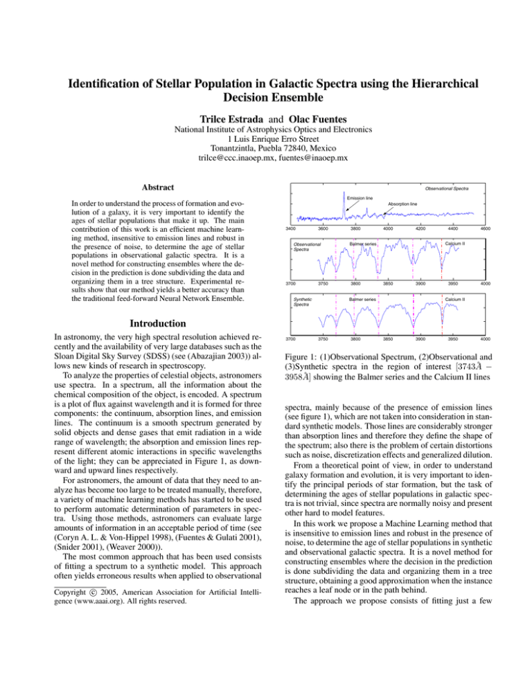
of the light; they can be appreciated in Figure 1, as downward and upward lines respectively.
For astronomers, the amount of data that they need to analyze has become too large to be treated manually, therefore,
a variety of machine learning methods has started to be used
to perform automatic determination of parameters in spectra. Using those methods, astronomers can evaluate large
amounts of information in an acceptable period of time (see
(Coryn A. L. & Von-Hippel 1998), (Fuentes & Gulati 2001),
(Snider 2001), (Weaver 2000)).
The most common approach that has been used consists
of fitting a spectrum to a synthetic model. This approach
often yields erroneous results when applied to observational
c 2005, American Association for Artificial IntelliCopyright gence (www.aaai.org). All rights reserved.
3700
3750
3800
3850
3900
3950
4000
Figure 1: (1)Observational Spectrum, (2)Observational and
(3)Synthetic spectra in the region of interest [3743Å −
3958Å] showing the Balmer series and the Calcium II lines
spectra, mainly because of the presence of emission lines
(see figure 1), which are not taken into consideration in standard synthetic models. Those lines are considerably stronger
than absorption lines and therefore they define the shape of
the spectrum; also there is the problem of certain distortions
such as noise, discretization effects and generalized dilution.
From a theoretical point of view, in order to understand
galaxy formation and evolution, it is very important to identify the principal periods of star formation, but the task of
determining the ages of stellar populations in galactic spectra is not trivial, since spectra are normally noisy and present
other hard to model features.
In this work we propose a Machine Learning method that
is insensitive to emission lines and robust in the presence of
noise, to determine the age of stellar populations in synthetic
and observational galactic spectra. It is a novel method for
constructing ensembles where the decision in the prediction
is done subdividing the data and organizing them in a tree
structure, obtaining a good approximation when the instance
reaches a leaf node or in the path behind.
The approach we propose consists of fitting just a few
lines of the spectrum that contain the information related to
the age of the stellar populations. It has the additional advantage that it does not use regions with strong emission lines.
Our experimental results show the efficacy of the proposed
method applied to a difficult pattern recognition problem.
The organization of the remainder of this paper is as follows: Section 2 describes the data used in the experiments.
Section 3 describes the process used to characterize the spectra. Section 4 presents the ensemble method used to predict
the age of stellar populations. Section 5 presents experimental results using synthetic and observational spectra, and
Section 6 presents conclusions and future work.
Data
The spectra are defined by 2 vectors; the first one is the
wavelength and the second is the amount of flux in that
point, the difference between a specific wavelength and the
next is the sampling rate; the measurement unit used in astronomy for denoting the wavelength is the Angstrom (abbreviated Å) and represents 1 × 10−13 meter.
The observational data consists of 1157 galactic spectra
obtained from the Sloan Digital Sky Survey (see (Abazajian
2003)) with a sampling rate of 1Å and a range from 3435Å
to 8315Å.
A galactic spectrum is composed of stars, nebula and interstellar dust. In general terms an observational spectrum
can be considered as the combination of a few main stellar populations. Those populations are formed by stars with
similar cinematic properties, ages and chemical composition. Thus, to analyze the observational spectra, we generated simulated galactic spectra as the sum of three synthetic
models of stellar populations with different ages. In order
to make the simulated data as similar to the observational
galactic spectra as possible, we added noise and gaussian
smoothing.
→
The synthetic models (−
m x ) are composed by 14 high resolution spectra (see (Cerviño M. 2000)) at 0.3Å sampling
and a range from 3000Å to 6900Å. The experiments were
calibrated using three populations with different ages and
proportions:
• age1: A young population with ages between 107.0 and
107.6 years, representing a starburst component, five spectra.
• age2: An intermediate population with ages between
108.0 and 108.6 years, four spectra.
• age3: An old population with ages between 109.0 and
109.6 years, representing the bulge component, five spectra.
In this work we focused on five spectral lines that encode
most of the information related to the age of the stellar populations; those lines are the Balmer series and Calcium II
(see figure 1) that are characteristic of the young and the old
stellar populations respectively. This subset of the spectra
consist of 717 points with wavelength between 3743Å and
3958Å.
Generation of Simulated Spectra. A simulated spec−
→
trum S sim is a combination of synthetic models that rep-
resents a galaxy with three principal stellar populations of
different ages. Define Mmodels the matrix containing the 14
synthetic models; as
⎞
⎛ −
→
m1
⎟
⎜
(1)
Mmodels ∈ R14x717 = ⎝ ... ⎠
−
→
m 14
1x5 −
1x4
−
→
→
−
→
p1 ∈ R , p2 ∈ R
and p3 ∈ R1x5 are vectors representing the proportion of the stellar populations: age1,
age2 and age3 respectively, each with just one non-zero element that represents one specific age in the simulated galactic spectra, where:
3 −
→
pi = 1
(2)
i=1
−
−→ is the vector that results of concatenating −
→
→
ages
p1 , −
p2 and
−
→
p3 . It contains the proportions of ages, with just three nonzero elements:
→
→
→
−
−→ ∈ R1x14 = (−
p1 , −
p2 , −
p3 )
ages
(3)
Then Ssim is constructed as follows:
−
→
→
−→ ∗ Mmodels ) + −
S sim = smooth(−
ages
S noise (4)
−
→
where S noise ∈ R1x717 is a random vector of the same
→
−
size as S sim that represents gaussian noise. The function
smooth is used for smoothing the spectra simulating the
limited resolution of the observations; it uses gaussian window filtering with a standard deviation of 0.70 and a window
size ranging from 5 to 11.
−→ The
Each simulated galactic spectrum is defined by −
ages.
pattern recognition task consists of predicting the non-zero
elements that best fit the line profiles, producing a resultant
spectrum that is as similar to the observed one as possible.
Data properties. Spectra are not chaotic signals, on the
contrary, a spectrum has a defined behavior depending on
its spectral parameters. In a spectrum there are several lines
that always appear in certain wavelengths; those lines can be
weaker or stronger depending on the structure of the object.
In this case, the width of the Calcium line and the lines in
the Balmer series encode the relevant information about the
age of its populations.
As we can see in Table 1, the resolution in the synthetic
and the observational spectra are different, and there are
emission lines in the observational spectra that are not considered in the synthetic ones. These differences are very important, and they complicate the task of fitting the whole
spectrum, that is the reason we decide to fit just few lines
where there are not strong emission lines.
To characterize the properties of the five lines, we extract
the width of the lines in 12 regions; it is a key step in the
preprocessing, because we eliminate most of the noise effects and maintain the relevant information about each line.
The widths are the features that we use to characterize each
spectrum and make the age prediction. In this stage we can
eliminate most of the noise in the spectrum because we do
Figure 2: Tree structure of the Hierarchical Decision Ensemble
not focus on each flux point, which could be contaminated,
but on general features such as the spectrum shape in a specific area. We extract 12 widths per line in 5 lines, obtaining
a total of 60 features.
Hierarchical Decision Ensemble (HDE)
The hierarchical ensemble (figure 2) is a tree-based algorithm (see (Quinlan 1986)); in each step we train a classifier
using a training set and predict the parameters for a validation set. The spectra corresponding to the predicted parameters are reconstructed and compared with the validation set.
The predictions of those spectra that have an error that is
smaller than a predefined threshold are accepted, and those
spectra that are not accepted are added to the training set
along with the reconstructed spectra; this new training set is
divided into two subsets using a clustering algorithm, then
each subgroup is used to train new classifiers in the next
level of the tree (see figure 3), this is done until all the errors
are lower than the threshold or until a predefined number of
levels is reached.
In the prediction stage, each instance in the test set, is
evaluated for the first node using the trained classifier. The
prediction is employed to reconstruct a simulated spectrum.
If the RMS error in the comparison is lower than a predefined threshold, the prediction is accepted. If the error is
higher than the threshold, the trained divider in the node is
used to determine the next path of the instance. This process
is repeated until the instance obtains an accepted prediction
Table 1: Summary of properties of the data test
P ROPERTY
S YNTHETIC
O BSERVATIONAL
Number of spectra
3600
1155
Resolution
0.3Å
1Å
Spectral range
[3435-8315]Å
[3000-6900]Å
Emission lines
No
Yes
Noise
10%
Un known
Number of features
60
60
Figure 3: Internal node in HDE
or until it reaches a leaf node. The prediction and the error
produced by each node are stored to make a final decision at
the end of the process.
Feature Selection. We calculate the inter-class and intraclass variations for each age. These measurements are used
to analyze the data behavior and we prefer those features that
have low intra-class variation and high inter-class variation.
Let Xj ∈ Rnj ×m be the matrix of instances relevant to
→
the class j where −
µ j is the matrix of means in class j and
µ is the matrix of total means, nj is the total number of instances in class j and c is the total number of classes (see
(Fisher 1936)).
Define E ∈ Rm×m as the inter-class variation and I ∈
Rm×m as the intra-class variation:
E=
c
→
→
nj · (−
µ j − µ)(−
µ j − µ)T
(5)
j=i
I=
c →
→
µ j )(Xj − −
µ j )T
(Xj − −
(6)
j=1
Classifier. This module is independent of the algorithm,
in this paper we have used standard feedforward neural networks and locally weighted linear regression, but we could
use any supervised machine learning algorithm. Neural networks were chosen because of their speed at prediction time
and generalization ability and LWR was introduced to add
diversity to the tree. The classifier is trained using half of
the total data, leaving a subset for validating its generalization ability in the specific level of the tree.
Error Estimation and Data Set Regeneration. The error estimation process uses the reconstructed galactic spectra
f (pred) and calculates its difference from the spectra in the
test set. The resulting error is compared with a threshold,
after that, we modify the data set adding those reconstructed
spectra that have an RMS error higher than the threshold
and removing those spectra in the test set that have an RMS
error lower than the threshold. Both thresholds were set experimentally to accept about 15% of the predictions and to
add about 40% of new reconstructed spectra.
Divider. In the divider module we make a clustering
process; this stage is independent of the algorithm, too. In
this work we use k-means (Alsabti & Singh 1998), but it
could be done using any clustering algorithm. Each cluster
is then passed to the next level of the tree to train a new classifier. For the experiments we use k = 2 for simplicity and
to generate small trees, but this parameter can be modified
depending on the problem.
Experimental Results
In this work we made four experiments, the task was fitting
the five lines of the spectra and predicting the parameters
corresponding to the age and proportion of each stellar population. Using the predicted parameters we reconstruct the
suggested spectrum and compare it with the original; considering that a prediction is better than another when the reconstructed spectrum produced by this prediction is more
similar to the original than the reconstructed spectrum produced by the other prediction. Bellow we will explain briefly
the experiments.
ANN-E Feedforward-Backpropagation Neural Network
Ensemble. It consists of 5 classifiers trained independently, using five different data sets of 3600 spectra, and
combining their predictions by average.
LWR-E Locally Weighted Regression Ensemble. It is
made in a similar way as the ANN-E.
ANN-LWR Heterogeneous Ensemble. It is formed by 3
classifiers trained with neural networks and 2 classifiers
trained with locally weighted regression.
HDE Hierarchical Decision Ensemble.
Combining
Feedforward-Backpropagation Neural Networks and
Locally Weighted Regression nodes; restricting the tree
growth to 5 levels to obtain small trees keeping the
balance between accuracy and efficiency.
We compared the performance of the HDE with the three
ensembles made in a traditional way; finding that the generalization ability of the HDE was better than the other experiments realized here for the presented problem. The summary of results is shown in Table 2 and Table 3.
Table 3: RMS-Error obtained in observational spectra using
traditional ensembles and the HDE
O BSERVATIONAL GALACTIC
A LGORITHM
SPECTRA
Profile fitting Reconstructed spectra
ANN-E
0.348
0.411
LWR-E
0.323
0.425
ANN-LWR
0.357
0.467
HDE
0.291
0.321
we calculate the Root Mean Square Error for each instance
and average all the errors to obtain a confidence measurement. In a secondary stage we used a test set consisting of
3600 new examples which have not been seen before by the
algorithm, with parameters generated randomly. Both experiments were similar in precision. Here we present the
average of results obtained in the two stages. To predict the
parameters in the observational galactic spectra we used the
ensembles generated in the previous step.
The prediction time required for the traditional ensembles
is about 1.1 seconds per spectra and the time consumed by
the HDE is about 1.7 seconds per spectra. Although the time
taken by HDE is higher than the time taken by the normal
ensembles, the errors in the profiles and the reconstructed
spectra using the HDE prediction are better than the best
obtained using the traditional ensembles prediction, as we
can see in Figure 4. As expected, the RMS-error is higher
for the observational spectra than for the synthetic spectra,
because the profiles of the synthetic lines are better defined
and there are no emission lines inside the absorption lines as
in the observational spectra.
ANN−E
1
0.5
0
−0.5
Real
Synthetic
−1
3740
Table 2: RMS-Error obtained in synthetic galactic spectra
using traditional ensembles and the HDE
P REDICTION S YNTHETIC GALACTIC
A LGORITHM
T IME
SPECTRA
Profile fitting
ANN-E
0.8 sec.
0.0451
LWR-E
1.5 sec.
0.0435
ANN-LWR
1.1 sec.
0.0447
HDE
1.7 sec.
0.0431
For the synthetic data we generated 10800 simulated
galactic spectra and tested the methods in two stages, in the
first one, we used ten fold cross validation, where we divide the data into 10 subsets of equal size, train the classifier
10 times, each time leaving out one of the subsets and using it for testing the algorithm. At the end of the process
3760
3780
3800
3820
3840
3860
3880
3900
3920
3940
3880
3900
3920
3940
HET−HDE
1
Real
Synthetic
0.5
0
−0.5
−1
3740
3760
3780
3800
3820
3840
3860
Figure 4: Fitting in an observational spectrum
Conclusions and Future Work
We have introduced a novel method for constructing ensembles using the divide and conquer principle, which is specially effective when there are several distinct subgroups that
share a behavior.
To determine the age of stellar populations in synthetic
and observational galactic spectra, the accuracy of the HDE
is better than the one obtained using traditional ensemble
methods.
We presented an efficient machine learning method for
identification of ages in galactic spectra, which is robust in
the presence of noise, and in addition is insensitive to strong
emission lines.
For future work we will experiment with different algorithms for the classifier and the divider modules and we will
examine the behavior of the HDE using different data sets.
References
Abazajian, K. e. a. 2003. The first data release of the sloan
digital sky survey. The Astronomical Journal 126:2081–
2086.
Alsabti, K., R. S., and Singh, V. 1998. An efficient kmeans clustering algorithm. In First Workshop on HighPerformance Data Mining.
Cerviño M., e. a. 2000. Evolutionary synthesis models for
young star forming regions that compute the stellar energy
dispersion and distribution. A&A 363.
Coryn A. L., Bailer-Jones, I. M., and Von-Hippel, T. 1998.
Automated classification of stellar spectra ii. Monthly Notices of the Royal Astronomical Society.
Fisher, R. 1936. The use of multiple measures in taxonomic problems. Ann. Eugenics 7:179–188.
Fuentes, O., and Gulati, R. K. 2001. Prediction of stellar atmospheric parameters using neural networks and instancebased learning. Experimental Astronomy 12:21–31.
Quinlan, J. R. 1986. Induction of decision trees. Machine
Learning 1:81–106.
Snider, S., e. a. 2001. Three-dimensional spectral classification of low-metallicity stars using artificial neural networks. The Astrophisical Journal 562:528–548.
Weaver, W. 2000. Spectral classification of unresolved
binary stars with artificial neural networks. The Astrophysical Journal 541:298–305.