The Optimality of Naive Bayes
Harry Zhang
Faculty of Computer Science
University of New Brunswick
Fredericton, New Brunswick, Canada
E3B 5A3
email: hzhang@unb.ca
Abstract
Naive Bayes is one of the most efficient and effective
inductive learning algorithms for machine learning and
data mining. Its competitive performance in classification is surprising, because the conditional independence
assumption on which it is based, is rarely true in realworld applications. An open question is: what is the
true reason for the surprisingly good performance of
naive Bayes in classification?
In this paper, we propose a novel explanation on the
superb classification performance of naive Bayes. We
show that, essentially, the dependence distribution; i.e.,
how the local dependence of a node distributes in each
class, evenly or unevenly, and how the local dependencies of all nodes work together, consistently (supporting a certain classification) or inconsistently (canceling each other out), plays a crucial role. Therefore,
no matter how strong the dependences among attributes
are, naive Bayes can still be optimal if the dependences
distribute evenly in classes, or if the dependences cancel each other out. We propose and prove a sufficient
and necessary conditions for the optimality of naive
Bayes. Further, we investigate the optimality of naive
Bayes under the Gaussian distribution. We present and
prove a sufficient condition for the optimality of naive
Bayes, in which the dependence between attributes do
exist. This provides evidence that dependence among
attributes may cancel out each other. In addition, we
explore when naive Bayes works well.
Rule, the probability of an example E = (x1 , x2 , · · · , xn )
being class c is
p(c|E) =
E is classified as the class C = + if and only if
fb (E) =
c 2004, American Association for Artificial IntelliCopyright gence (www.aaai.org). All rights reserved.
p(C = +|E)
≥ 1,
p(C = −|E)
(1)
where fb (E) is called a Bayesian classifier.
Assume that all attributes are independent given the value
of the class variable; that is,
p(E|c) = p(x1 , x2 , · · · , xn |c) =
n
p(xi |c),
i=1
the resulting classifier is then:
n
fnb (E) =
p(C = +) p(xi |C = +)
.
p(C = −) i=1 p(xi |C = −)
(2)
The function fnb (E) is called a naive Bayesian classifier,
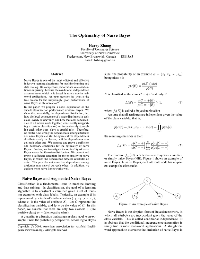
or simply naive Bayes (NB). Figure 1 shows an example of
naive Bayes. In naive Bayes, each attribute node has no parent except the class node.
Naive Bayes and Augmented Naive Bayes
Classification is a fundamental issue in machine learning
and data mining. In classification, the goal of a learning
algorithm is to construct a classifier given a set of training examples with class labels. Typically, an example E is
represented by a tuple of attribute values (x1 , x2 , , · · · , xn ),
where xi is the value of attribute Xi . Let C represent the
classification variable, and let c be the value of C. In this
paper, we assume that there are only two classes: + (the
positive class) or − (the negative class).
A classifier is a function that assigns a class label to an example. From the probability perspective, according to Bayes
p(E|c)p(c)
.
p(E)
C
A1
A2
A3
A4
Figure 1: An example of naive Bayes
Naive Bayes is the simplest form of Bayesian network, in
which all attributes are independent given the value of the
class variable. This is called conditional independence. It
is obvious that the conditional independence assumption is
rarely true in most real-world applications. A straightforward approach to overcome the limitation of naive Bayes is
to extend its structure to represent explicitly the dependencies among attributes. An augmented naive Bayesian network, or simply augmented naive Bayes (ANB), is an extended naive Bayes, in which the class node directly points
to all attribute nodes, and there exist links among attribute
nodes. Figure 2 shows an example of ANB. From the view
of probability, an ANB G represents a joint probability distribution represented below.
pG (x1 , · · · , xn , c) = p(c)
n
p(xi |pa(xi ), c),
(3)
i=1
where pa(xi ) denotes an assignment to values of the parents of Xi . We use pa(Xi ) to denote the parents of Xi .
ANB is a special form of Bayesian networks in which no
node is specified as a class node. It has been shown that any
Bayesian network can be represented by an ANB (Zhang &
Ling 2001). Therefore, any joint probability distribution can
be represented by an ANB.
C
A1
A2
A3
A4
Figure 2: An example of ANB
When we apply a logarithm to fb (E) in Equation 1, the
resulting classifier log fb (E) is the same as fb (E), in the
sense that an example E belongs to the positive class, if and
only if log fb (E) ≥ 0. fnb in Equation 2 is similar. In this
paper, we assume that, given a classifier f , an example E
belongs to the positive class, if and only if f (E) ≥ 0.
Related Work
Many empirical comparisons between naive Bayes and modern decision tree algorithms such as C4.5 (Quinlan 1993)
showed that naive Bayes predicts equally well as C4.5 (Langley, Iba, & Thomas 1992; Kononenko 1990; Pazzani 1996).
The good performance of naive Bayes is surprising because
it makes an assumption that is almost always violated in realworld applications: given the class value, all attributes are
independent.
An open question is what is the true reason for the surprisingly good performance of naive Bayes on most classification tasks? Intuitively, since the conditional independence
assumption that it is based on is almost never hold, its performance may be poor. It has been observed that, however,
its classification accuracy does not depend on the dependencies; i.e., naive Bayes may still have high accuracy on the
datasets in which strong dependencies exist among attributes
(Domingos & Pazzani 1997).
Domingos and Pazzani (Domingos & Pazzani 1997)
present an explanation that naive Bayes owes its good performance to the zero-one loss function. This function defines the error as the number of incorrect classifications
(Friedman 1996). Unlike other loss functions, such as the
squared error, the zero-one loss function does not penalize
inaccurate probability estimation as long as the maximum
probability is assigned to the correct class. This means that
naive Bayes may change the posterior probabilities of each
class, but the class with the maximum posterior probability
is often unchanged. Thus, the classification is still correct,
although the probability estimation is poor. For example, let
us assume that the true probabilities p(+|E) and p(−|E) are
0.9 and 0.1 respectively, and that the probability estimates
p(+|E) and p(−|E) produced by naive Bayes are 0.6 and
0.4. Obviously, the probability estimates are poor, but the
classification (positive) is not affected.
Domingos and Pazzani’s explanation (Domingos & Pazzani 1997) is verified by the work of Frank et al. (Frank et
al. 2000), which shows that the performance of naive Bayes
is much worse when it is used for regression (predicting a
continuous value). Moreover, evidence has been found that
naive Bayes produces poor probability estimates (Bennett
2000; Monti & Cooper 1999).
In our opinion, however, Domingos and Pazzani (Domingos & Pazzani 1997)’s explanation is still superficial as it
does not uncover why the strong dependencies among attributes could not flip the classification. For the example
above, why the dependencies could not make the probability
estimates p(+|E) and p(−|E) produced by naive Bayes be
0.4 and 0.6? The key point here is that we need to know how
the dependencies affect the classification, and under what
conditions the dependencies do not affect the classification.
There has been some work to explore the optimality of
naive Bayes (Rachlin, Kasif, & Aha 1994; Garg & Roth
2001; Roth 1999; Hand & Yu 2001), but none of them give
an explicit condition for the optimality of naive Bayes.
In this paper, we propose a new explanation that the classification of naive Bayes is essentially affected by the dependence distribution, instead by the dependencies among
attributes. In addition, we present a sufficient condition for
the optimality of naive Bayes under the Gaussian distribution, and show theoretically when naive Bayes works well.
A New Explanation on the Superb
Classification Performance of Naive Bayes
In this section, we propose a new explanation for the surprisingly good classification performance of naive Bayes. The
basic idea comes from the observation as follows. In a given
dataset, two attributes may depend on each other, but the
dependence may distribute evenly in each class. Clearly, in
this case, the conditional independence assumption is violated, but naive Bayes is still the optimal classifier. Further, what eventually affects the classification is the combination of dependencies among all attributes. If we just
look at two attributes, there may exist strong dependence between them that affects the classification. When the dependencies among all attributes work together, however, they
may cancel each other out and no longer affect the classification. Therefore, we argue that it is the distribution of dependencies among all attributes over classes that affects the
classification of naive Bayes, not merely the dependencies
themselves.
Before discussing the details, we introduce the formal
definition of the equivalence of two classifiers under zeroone loss, which is used as a basic concept.
Definition 1 Given an example E, two classifiers f1 and f2
are said to be equal under zero-one loss on E, if f1 (E) ≥ 0
.
if and only if f2 (E) ≥ 0, denoted by f1 (E) = f2 (E). If for
.
every example E in the example space, f1 (E) = f2 (E), f1
and f2 are said to be equal under zero-one loss, denoted by
.
f1 = f2 .
Local Dependence Distribution
As discussed in the section above, ANB can represent any
joint probability distribution. Thus we choose an ANB as
the underlying probability distribution. Our motivation is to
find out under what conditions naive Bayes classifies exactly
the same as the underlying ANB.
Assume that the underlying probability distribution is an
ANB G with two classes {+, −}, and the dependencies
among attributes are represented by the arcs among attribute
nodes. For each node, the influence of its parents is quantified by the correspondent conditional probabilities. We call
the dependence between a node and its parents local dependence of this node. How do we measure the local dependence of a node in each class? Naturally, the ratio of the
conditional probability of the node given its parents over the
conditional probability of the node without the parents, reflects how strong the parents affect the node in each class.
Thus we have the following definition.
Definition 2 For a node X on ANB G, the local dependence
derivative of X in classes + and − are defined as below.
p(x|pa(x), +)
p(x|+)
p(x|pa(x), −)
dd−
.
G (x|pa(x)) =
p(x|−)
dd+
G (x|pa(x)) =
(4)
(5)
Essentially, dd+
G (x|pa(x)) reflects the strength of the local dependence of node X in class +, which measures the
influence of X’s local dependence on the classification in
class +. dd−
G (x|pa(x)) is similar. Further, we have the following results.
1. When X has no parent, then
−
dd+
G (x|pa(x)) = ddG (x|pa(x)) = 1.
2. When dd+
G (x|pa(x)) ≥ 1, X’s local dependence in class
+ supports the classification of C = +. Otherwise, it
supports the classification of C = −. Similarly, when
dd−
G (x|pa(x)) ≥ 1, A’s local dependence in class − supports the classification of C = −. Otherwise, it supports
the classification of C = +.
Intuitively, when the local dependence derivatives in both
classes support the different classifications, the local dependencies in the two classes cancel partially each other out, and
the final classification that the local dependence supports, is
the class with the greater local dependence derivative. Another case is that the local dependence derivatives in the two
classes support the same classification. Then, the local dependencies in the two classes work together to support the
classification.
The discussion above shows that the ratio of the local dependence derivatives in both classes ultimately determines
which classification the local dependence of a node supports.
Thus we have the following definition.
Definition 3 For a node X on ANB G, the local dependence
derivative ratio at node X, denoted by ddrG (x) is defined
below:
dd+
G (x|pa(x))
ddrG (x) = −
.
(6)
ddG (x|pa(x))
From the above definition, ddrG (x) quantifies the influence of X’s local dependence on the classification. Further,
we have the following results.
1. If X has no parents, ddrG (x) = 1.
−
2. If dd+
G (x|pa(x)) = ddG (x|pa(x)), ddrG (x) = 1. This
means that x’s local dependence distributes evenly in
class + and class −. Thus, the dependence does not affect
the classification, no matter how strong the dependence
is.
3. If ddrG (x) > 1, X’s local dependence in class + is
stronger than that in class −. ddrG (x) < 1 means the
opposite.
Global Dependence Distribution
Now let us explore under what condition an ANB works exactly the same as its correspondent naive Bayes. The following theorem establishes the relation of an ANB and its
correspondent naive Bayes.
Theorem 1 Given an ANB G and its correspondent naive
Bayes Gnb (i.e., remove all the arcs among attribute nodes
from G) on attributes X1 , X2 , ..., Xn , assume that fb and
fnb are the classifiers corresponding to G and Gnb , respectively. For a given example E = (x1 , x2 , · · ·, xn ), the equation below is true.
fb (x1 , x2 , ..., xn ) = fnb (x1 , x2 , ..., xn )
n
ddrG (xi ), (7)
i=1
n
where i=1 ddrG (xi ) is called the dependence distribution
factor at example E, denoted by DFG (E).
Proof: According to Equation 3, we have:
fb (x1 , · · · , xn ) =
n
p(+) p(xi |pa(xi ), +)
p(−)
p(xi |pa(xi ), −)
i=1
=
n
n
p(+) p(xi |+) p(xi |pa(xi ), +)p(xi |−)
p(−)
i=1
p(xi |−)
i=1
p(xi |pa(xi ), −)p(xi |+)
=
fnb (E)
n
ddr+ (xi |pa(xi ))
i=1
=
fnb (E)
Theorem 2 represents a sufficient and necessary condition
for the optimality of naive Bayes on an example E. If for
.
each example E in the example space, fb (E) = fnb (E);
.
i.e., fb = fnb , then naive Bayes is globally optimal.
G
n
−
ddrG
(xi |pa(xi ))
ddrG (xi )
i=1
=
Conditions for the Optimality of Naive Bayes
DFG (E)fnb (E)
(8)
From Theorem 1, we know that, in fact, it is the dependence distribution factor DFG (E) that determines the difference between an ANB and its correspondent naive Bayes
in the classification. Further, DFG (E) is the product of local
dependence derivative ratios of all nodes. Therefore, it reflects the global dependence distribution (how each local dependence distributes in each class, and how all local dependencies work together). For example, when DFG (E) = 1,
G has the same classification as Gnb on E. In fact, it is
not necessary to require DFG (E) = 1, in order to make
an ANB G has the same classification as its correspondent
naive Bayes Gnb , as shown in the theorem below.
Theorem 2 Given an example E = (x1 , x2 , ..., xn ), an
ANB G is equal to its correspondent naive Bayes Gnb un.
der zero-one loss; i.e., fb (E) = fnb (E) (Definition 1), if
and only if when fb (E) ≥ 1, DFG (E) ≤ fb (E); or when
fb (E) < 1, DFG (E) > fb (E).
Proof: The proof is straightforward by apply Definition
1 and Theorem 1.
From Theorem 2, if the distribution of the dependences
among attributes satisfies certain conditions, then naive
Bayes classifies exactly the same as the underlying ANB,
even though there may exist strong dependencies among attributes. Moreover, we have the following results:
In Section , we proposed that naive Bayes is optimal if the
dependences among attributes cancel each other out. That
is, under circumstance, naive Bayes is still optimal even
though the dependences do exist. In this section, we investigate naive Bayes under the multivariate Gaussian distribution and prove a sufficient condition for the optimality
of naive Bayes, assuming the dependences among attributes
do exist. That provides us with theoretic evidence that the
dependences among attributes may cancel each other out.
Let us restrict our discussion to two attributes X1 and X2 ,
and assume that the class density is a multivariate Gaussian
in both the positive and negative classes. That is,
−1
+ T
1
(x−µ+ )
+
1 1/2 e− 2 (x−µ )
p(x1 , x2 , +) =
,
2π|
p(x1 , x2 , −) =
3. The dependencies in an ANB flip (change) the classification of its correspondent naive Bayes, only if the condition
given by Theorem 2 is no longer true.
1
|
|
−
−1
(x−µ− )T
2
e
1/2
−1
−
(x−µ− )
,
where x = (x1 , x2 ), + and − are the covariance matri
ces in the positive and negative classes respectively, | − |
−1
and | + | are the determinants of − and + , + and
−1
+
+
+
− are the inverses of
− and
+ ; µ = (µ1 , µ2 ) and
−
−
+
−
−
µ = (µ1 , µ2 ), µi and µi are the means of attribute Xi in
the positive and negative classes respectively, and (x−µ+ )T
and (x − µ− )T are the transposes of (x − µ+ ) and (x − µ− ).
We assume
that
have a common covariance
two classes
matrix + = − = , and X1 and X2 have the same
variance σ in both classes. Then, when applying a logarithm
to the Bayesian classifier, defined in Equation 1, we obtain
the classifier fb below.
1. When DFG (E) = 1, the dependencies in ANB G has no
influence on the classification. That is, the classification
of G is exactly the same as that of its correspondent naive
Bayes Gnb . There exist three cases for DFG (E) = 1.
• no dependence exists among attributes.
• for each attribute X on G, ddrG (x) = 1; that is, the local distribution of each node distributes evenly in both
classes.
• the influence that some local dependencies support
classifying E into C = + is canceled out by the influence that other local dependences support classifying
E into C = −.
.
2. fb (E) = fnb (E) does not require that DFG (E) = 1.
The precise condition is given by Theorem 2. That explains why naive Bayes still produces accurate classification even in the datasets with strong dependencies among
attributes (Domingos & Pazzani 1997).
2π|
+
fb (x1 , x2 ) = log
=−
+xT
p(x1 , x2 , +)
p(x1 , x2 , −)
−1 +
1 +
−
(µ
+
µ
)
(µ − µ− )
σ2
−1
(µ+ − µ− ).
Then, because of the conditional independence assumption, we have the correspondent naive Bayesian classifier
fnb
fnb (x1 , x2 ) =
Assume that
1 +
1 +
−
(µ − µ−
1 )x1 + 2 (µ2 − µ2 )x2 .
σ2 1
σ
=
σ
σ12
σ12
σ
.
X1 and X2 are independent if σ12 = 0. If σ = σ12 , we
have
−σ
σ12
−1
σ 2 −σ 2
σ 2 −σ 2
=
12
σ12
2 −σ 2
σ12
12
−σ
2 −σ 2
σ12
.
Note that, an example E is classified into the positive class
by fb , if and only if fb ≥ 0. fnb is similar. Thus, when fb or
fnb is divided by a non-zero positive constant, the resulting
classifier is the same as fb or fnb . Then,
−
+
−
fnb (x1 , x2 ) = (µ+
1 − µ1 )x1 + (µ2 − µ2 )x2 ,
y
(9)
y=w1x+w2
and
fb (x1 , x2 ) =
1
−
+
−
= 2
(σ12 (µ+
2 − µ2 ) − σ(µ1 − µ1 ))x1
σ12 − σ 2
1
−
+
−
+ 2
(σ12 (µ+
1 − µ1 ) − σ(µ2 − µ2 ))x2
σ12 − σ 2
+a,
(10)
−1
where a = − σ12 (µ+ + µ− )
(µ+ − µ− ), a constant
independent of x.
For any x1 and x2 , naive Bayes has the same classification
as that of the underlying classifier if
fb (x1 , x2 )fnb (x1 , x2 ) ≥ 0.
(11)
That is,
1
−
+
−
+
− 2
2
((σ12 (µ+
1 − µ1 )(µ2 − µ2 ) − σ(µ1 − µ1 ) )x1
2
σ12
− σ2
−
+
−
+
− 2
2
+(σ12 (µ+
1 − µ1 )(µ2 − µ2 ) − σ(µ2 − µ2 ) )x2
−
+
−
+
− 2
+(2σ12 (µ+
1 − µ1 )(µ2 − µ2 ) − σ((µ1 − µ1 )
− 2
+(µ+
2 − µ2 ) ))x1 x2 )
−
+
−
+a(µ+
1 − µ1 )x1 + a(µ2 − µ2 )x2 ≥ 0
(12)
Equation 12 represents a sufficient and necessary condi.
tion for fnb (x1 , x2 ) = fb (x1 , x2 ). But it is too complicated.
+
−
−
Let (µ1 − µ1 ) = (µ+
2 − µ2 ). Equation 12 is simplified as
below.
(13)
w1 (x1 + x2 )2 + w2 (x1 + x2 ) ≥ 0,
(µ+ −µ− )2
+
−
1
1
where w1 =
σ12 +σ , and w2 = a(µ1 − µ1 ). Let
x = x1 + x2 , and y = w1 (x1 + x2 )2 + w2 (x1 + x2 ). Figure
3 shows the area in which naive Bayes has the same classification with the target classifier. Figure 3 shows that, under
certain condition, naive Bayes is optimal.
The following theorem presents a sufficient condition for
that naive Bayes works exactly as the target classifier.
.
Theorem 3 fb = fnb , if one of the following two conditions
is true:
−
−
+
1. µ+
1 = −µ2 , µ1 = −µ2 , and σ12 + σ > 0.
−
+
−
2. µ+
1 = µ2 , µ2 = µ1 , and σ12 − σ > 0.
µ+
1
−µ−
2,
µ−
1
−µ+
2,
x
Figure 3: Naive Bayes has the same classification with that
of the target classifier in the shaded area.
−
+
−
+
−
+
−
(2) If µ+
1 = µ2 , µ2 = µ1 , then (µ1 − µ1 ) = −(µ2 − µ2 ),
and a = 0. Thus, Equation 12 is simplified as below.
− 2
(µ+
1 − µ1 )
(x1 + x2 )2 ≥ 0,
σ12 − σ
(14)
It is obvious that Equation 14 is true for any x1 and x2 , if
.
σ12 − σ > 0. Therefore, fb = fnb .
Theorem 3 represents an explicit condition that naive
Bayes is optimal. It shows that naive Bayes is still optimal
under certain condition, even though the conditional independence assumption is violated. In other words, the conditional independence assumption is not the necessary condition for the optimality of naive Bayes. This provides evidence that the dependence distribution may play the crucial
role in classification.
Theorem 3 gives a strict condition that naive Bayes performs exactly as the target classifier. In reality, however, it is
not necessary to satisfy such a condition. It is more practical to explore when naive Bayes works well by investigating
what factors affect the performance of naive Bayes in classification.
Since under the assumption
that
have a com
two classes
mon covariance matrix + = − = , and X1 and X2
have the same variance σ in both classes, both fb and fnb
are linear functions, we can examine the difference between
them by measuring the difference between their coefficients.
So we have the following definition.
n
Definition
i=1 w1i xi + b and
n 4 Given classifiers f1 =
f2 =
w
x
+
c,
where
b
and
c
are
constants. The
2i
i
i=1
distance between two classifiers, denoted by D(f1 , f2 ), is
defined as below
n
D(f1 , f2 ) = (w1i − w2i )2 + (b − c)2 .
i=1
(µ+
1
− µ−
1)
− σ12 (µ+
Proof: (1) If
=
=
then
=
−
+
(µ+
2 − µ2 ). It is straightforward to verify that
−1 +
µ− )
(µ − µ− ) = 0. That is, for the constant a in
Equation 10, we have a = 0. Since σ12 + σ > 0, Equation
.
13 is always true for any x1 and x2 . Therefore, fb = fnb .
D(f1 , f2 ) = 0, if and only if they have the same coefficients. Obviously, naive Bayes will well approximate
the target classifier, if the distance between them are small.
Therefore, we can explore when naive Bayes works well by
observing what factors affect the distance.
2
When (σ12
− σ 2 ) > 0, fb can be simplified as below.
fb (x1 , x2 ) =
+(σ12 (µ+
1 −
Let r =
−
µ+
2 −µ2
−.
µ+
−µ
1
1
−
+
−
(σ12 (µ+
2 − µ2 ) − σ(µ1 − µ1 ))x1
−
+
−
2
µ1 ) − σ(µ2 − µ2 ))x2 + a(σ12
− σ 2 ),
−
If (µ+
1 − µ1 ) > 0, then
fnb (x1 , x2 ) = x1 + rx2 ,
and
fb (x1 , x2 ) = (σ12 r − σ)x1 + (σ12 − σr)x2 +
2
a(σ12
− σ2 )
− .
µ+
1 − µ1
Then,
D(fb , fnb ) = (1−σ12 r+σ)2 +(r−σ12 +σr)2 +
2
− σ 2 )2
a2 (σ12
− 2 .
(µ+
1 − µ1 )
(15)
−
It is easy to verify that, when (µ+
1 − µ1 ) < 0, we can
get the same D(fb , fnb ) in Equation 15. Similarly, when
2
− σ 2 ) < 0, we have
(σ12
D(fb , fnb ) = (1+σ12 r−σ)2 +(r+σ12 −σr)2 +
2
− σ 2 )2
a2 (σ12
.
+
2
(µ1 − µ−
1 )
(16)
From Equation 15 and 16, we see that D(fb , fnb ) is affected
by r, σ12 and σ. It is true that D(fb , fnb ) increases, as |r| increases. That means, the absolute ratio of distances between
two means of classes affect significantly the performance of
naive Bayes. More precisely, the less absolute ratio, the better performance of naive Bayes.
Conclusions
In this paper, we propose a new explanation on the classification performance of naive Bayes. We show that, essentially,
the dependence distribution; i.e., how the local dependence
of a node distributes in each class, evenly or unevenly, and
how the local dependencies of all nodes work together, consistently (support a certain classification) or inconsistently
(cancel each other out), plays a crucial role in the classification. We explain why even with strong dependencies, naive
Bayes still works well; i.e., when those dependencies cancel
each other out, there is no influence on the classification. In
this case, naive Bayes is still the optimal classifier. In addition, we investigated the optimality of naive Bayes under the
Gaussian distribution, and presented the explicit sufficient
condition under which naive Bayes is optimal, even though
the conditional independence assumption is violated.
References
Bennett, P. N. 2000. Assessing the calibration of Naive
Bayes’ posterior estimates. In Technical Report No. CMUCS00-155.
Domingos, P., and Pazzani, M. 1997. Beyond independence: Conditions for the optimality of the simple
Bayesian classifier. Machine Learning 29:103–130.
Frank, E.; Trigg, L.; Holmes, G.; and Witten, I. H. 2000.
Naive Bayes for regression. Machine Learning 41(1):5–15.
Friedman, J. 1996. On bias, variance, 0/1-loss, and the
curse of dimensionality. Data Mining and Knowledge Discovery 1.
Garg, A., and Roth, D. 2001. Understanding probabilistic
plassifiers. In Raedt, L. D., and Flach, P., eds., Proceedings of 12th European Conference on Machine Learning.
Springer. 179–191.
Hand, D. J., and Yu, Y. 2001. Idiots Bayes - not so stupid
after all? International Statistical Review 69:385–389.
Kononenko, I. 1990. Comparison of inductive and naive
Bayesian learning approaches to automatic knowledge acquisition. In Wielinga, B., ed., Current Trends in Knowledge Acquisition. IOS Press.
Langley, P.; Iba, W.; and Thomas, K. 1992. An analysis of
Bayesian classifiers. In Proceedings of the Tenth National
Conference of Artificial Intelligence. AAAI Press. 223–
228.
Monti, S., and Cooper, G. F. 1999. A Bayesian network
classifier that combines a finite mixture model and a Naive
Bayes model. In Proceedings of the 15th Conference on
Uncertainty in Artificial Intelligence. Morgan Kaufmann.
447–456.
Pazzani, M. J. 1996. Search for dependencies in Bayesian
classifiers. In Fisher, D., and Lenz, H. J., eds., Learning
from Data: Artificial Intelligence and Statistics V. Springer
Verlag.
Quinlan, J. 1993. C4.5: Programs for Machine Learning.
Morgan Kaufmann: San Mateo, CA.
Rachlin, J. R.; Kasif, S.; and Aha, D. W. 1994. Toward a better understanding of memory-based reasoning
systems. In Proceedings of the Eleventh International Machine Learning Conference. Morgan Kaufmann. 242–250.
Roth, D. 1999. Learning in natural language. In Proceedings of IJCAI’99. Morgan Kaufmann. 898–904.
Zhang, H., and Ling, C. X. 2001. Learnability of
augmented Naive Bayes in nominal domains. In Brodley, C. E., and Danyluk, A. P., eds., Proceedings of the
Eighteenth International Conference on Machine Learning. Morgan Kaufmann. 617–623.