Proceedings of the Twenty-Third AAAI Conference on Artificial Intelligence (2008)
Constrained Classification on Structured Data
Chi-Hoon Lee∗ Matthew Brown Russell Greiner
Shoajun Wang
Albert Murtha
{chihoon, mbrown, greiner}@cs.ualberta.ca
University of Alberta
Edmonton, Alberta, Canada
shaojun.wang@wright.edu
Wright State University
Dayton, Ohio, U.S.A
albertmu@cancerboard.ab.ca
Cross Cancer Institute
Edmonton, Alberta, Canada
Abstract
CRFs allow more complex dependencies, but their underlying computations are intractable. This is partly because
these systems simultaneously learn the parameters that optimize the label for each individual pixel by itself, and also
the parameters for jointly labelling pairs of adjacent pixels. Although approximation techniques have been adopted
to improve their computation efficiency, CRF variants, such
as Discriminative Random Fields (DRFs) still require costly
learning procedures (Kumar and Hebert 2003). Decoupled
Conditional Random Fields (DCRFs) presents an efficient
system by combining two classifiers that are each trained
separately (Lee, Greiner, and Zaı̈ane 2006). However, this
often reduces the accuracy of these systems.
This paper presents the PCRF system that can efficiently
use a simple discriminative classifier (LR) and still incorporate spatial compatibility, in a 2-D lattice. Our PCRF can be
viewed as a regularized i.i.d. discriminative classifier, where
the classification task is performed along with a regularized
term that explicitly considers dependencies of labels. In particular, PCRF first learns a classifier under the i.i.d. assumption, and then relaxes this i.i.d. assumption during testing.
Most standard learning algorithms, such as Logistic Regression (LR) and the Support Vector Machine (SVM),
are designed to deal with i.i.d. (independent and identically distributed) data. They therefore do not work effectively for tasks that involve non-i.i.d. data, such as
“region segmentation”. (Eg, the “tumor vs non-tumor”
labels in a medical image are correlated, in that adjacent pixels typically have the same label.) This has motivated the work in random fields, which has produced
classifiers for such non-i.i.d. data that are significantly
better than standard i.i.d.-based classifiers. However,
these random field methods are often too slow to be
trained for the tasks they were designed to solve. This
paper presents a novel variant, Pseudo Conditional Random Fields (PCRFs), that is also based on i.i.d. learners,
to allow efficient training but also incorporates correlations, like random fields. We demonstrate that this system is as accurate as other random fields variants, but
significantly faster to train.
Introduction
Radiation therapy planners need to know the location of the
tumor to determine what area to treat; this typically requires
labelling each pixel within an magnetic resonance (MR) image as either tumor or non-tumor. We could view this segmentor as a standard discriminative classifier, and try to apply standard techniques — eg, logistic regression (LR) or
support vector machine (SVM). Unfortunately, these systems work poorly for this task, as they assume that each
pixel’s label is independent of each other. This assumption is
not true, as spatially adjacent pixels typically have the same
label.
This has motivated many researchers to use systems that
can model and use complex dependencies among data instances, such as Markov Random Fields (MRFs) and Conditional Random Fields (CRFs) (Kumar and Hebert 2003;
Lee et al. 2007). This is not without costs, however. For instance, an MRF assumes that the observations are conditionally independent given their class labels; this clearly compromises their expressibility and hence their performance.
Pseudo Conditional Random Fields – PCRFs
Let X be an observed input image, where the observation
at pixel i is represented by xi , i ∈ S, where S is the set
of observed image pixels. Let Y be joint set of labels over
all pixels of an image. For simplicity we assume yi at pixel
i ∈ S is binary yi ∈ {−1, 1}. For instance, X might be
a magnetic resonance image of a brain and Y is a joint labelling over all pixels that indicates whether each pixel is
normal or a tumor.
Q We want to find the most-likely labelling
Pθ ( Y | X ) = i∈S Pθ ( yi | X, Y − yi ). Given feature vectors (observations) xi for each pixel i as well as the class
label yj for each neighboring pixel j ∈ Ni , the PCRF formulation then defines
Pθ ( yi | xi , xNi , yNi )
Q
= ψθ (xi , yi ) × j∈Ni φo (xi , xj ) × φc (yi , yj )
(1)
where the potential functions φo (xi , xj ) quantifies the similarity of the feature vectors for pixels i and j, and φc (yi , yj )
models the interactions between the two class labels yi and
yj . The system designer can adjust φc (.) to alter the degree of continuity with respect to class labels expected by the
∗
Much of this work done while working at Yahoo!
c 2008, Association for the Advancement of Artificial
Copyright Intelligence (www.aaai.org). All rights reserved.
1812
model; e.g., if φc gives high weight when neighboring pixels share the same class label, then PCRF will prefer having
the same class labels among neighboring pixels. Alternatively, setting φo ≡ 1 and φc ≡ 1 would remove all spatial
dependencies, leading to an i.i.d. classifier. Note we use a
fixed pair of potential functions: we set φo (xi , xj ) = xTi xj ,
as the similarity measure between neighboring pixels; note
this measure is maximal value when the two vectors are colinear. We also set φc (yi , yj ) = α if yi ≡ yj , and 1 − α
otherwise where α weighs the importance that adjacent pixels share the same label.
LR vs PCRF
85
90
85
80
log φ (xi , xj ) + log φo (yi , yj )
70
75
70
60
65
55
50
50
55
60
65
70
75
80
85
90
95
65
LR
70
75
80
85
LR
(a) Synthetic data sets
(b) MR image analysis
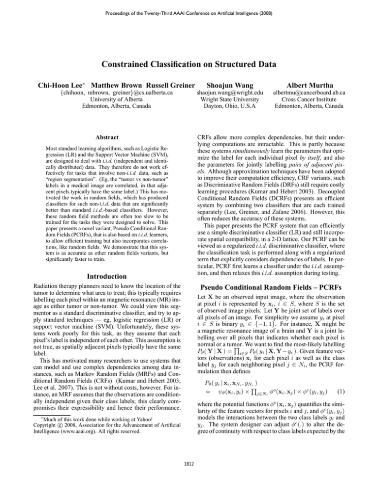
Figure 1: Jaccard Scores (percentage) for PCRF vs. LR
corrupted by Gaussian noise N (0, 1). For our real world
problem, datasets are MRI scans from 11 patients with brain
tumors; for each patient, we annotated each pixel with values based on three different MR imaging modalities: T1, T2,
and T1 with gadolinium contrast (“T1c”). Figure. 1 clearly
presents robustness of PCRF from synthetic images (a) and
brain tumor segmentation (b). Each point above the diagonal line indicates that PCRF produced a higher Jaccard
score (percentage) for a given test image. We also compare the PCRF’s performance with DRF’s for brain tumor
segmentation. On average, PCRF produced as accurate Jaccard scores (percentage) as DRFs: 73.69 versus 73.03, respectively. However, the PCRF’s learning time over 11 patients (38 seconds) is significantly more efficient than DRFs’
(1697 seconds average). Our PCRF was over 40 times faster
than the DRF (p < 10−37 , paired-samples t-tests). Refer
to (WEB ) for more details about experiments.
i∈S
c
75
65
Inference Our PCRF system incorporates the spatial correlations in the inference step. In general, our objective in
the inference process seeks Y∗ as:
X
Y∗ = arg max
log ψθ (xi , yi ) +
Y
PCRF
PCRF
80
Learning One key factor that constrains the form of typical CRF variant models is to compute exact expectations, as
required to learn parameters (Kumar and Hebert 2003).
Our PCRF defines ψθ (xi , y) as σ(θT xi ), where σ(t) =
1
1+exp(−t) corresponds to a standard local discriminative
classifier, Logistic Regression. This explicitly quantifies the
posterior probability of being in class y given observation
xi . Our PCRF learner is simple, and more efficient than
CRF variants, since we only need to fit the parameter θ for
a local potential function ψ(.). (Recall we hand-defined the
φc and φo functions.)
XX
LR vs PCRF
95
(2)
i∈S j∈Ni
Conclusion
The above equation requires searching an exponential search
space (i.e. 2|S| for binary case) to find an optimal Y∗ .
To efficiently solve (approximate) our objective, we formulate Eq. 2 using graph cuts algorithm that solves image
pixel classification tasks by minimizing an energy function
when spatial correlations among pixels are “independent”
of the observations; this involves using linear programming
to find the max-flow/min-cut on a graph in which nodes
correspond to pixels and edges correspond to connections
between neighboring pixels (Boykov, Veksler, and Zabih
1999). We reformulate this graph cuts approach to apply
to our PCRF framework (Eq. 2), in which neighbor relationships are dependent on both the labels and the observations
(feature vectors). Refer to (WEB )
As standard i.i.d. classifiers do not model interdependencies
of labels, they typically do very poorly for such tasks spatially constrained classification. In this paper, we proposed
an efficient model – Pseudo Conditional Random Fields
(PCRF) – that takes advantage of a typical discriminative
classifier (LR) when training, then relaxes the classifier’s
i.i.d. assumption during the inference. We demonstrate the
effectiveness and the efficiency of PCRFs from both synthetic and real world data sets — showing that its performance is comparable to state-of-the-art random field systems, but its training time is significantly more efficient.
References
Boykov, Y.; Veksler, O.; and Zabih, R. 1999. Fast approximate energy minimization via graph cuts. In ICCV.
Kumar, S., and Hebert, M. 2003. Discriminative fields for
modeling spatial dependencies in natural images. In NIPS.
Lee, C.-H.; Wang, S.; Jiao, F.; Schuurmans, D.; and
Greiner, R. 2007. Learning to model spatial dependency:
Semi-supervised discriminative random fields. In NIPS.
Lee, C.-H.; Greiner, R.; and Zaı̈ane, O. R. 2006. Efficient
spatial classification using decoupled conditional random
fields. In PKDD.
WEB. http://www.cs.ualberta.ca/∼chihoon/aaai2008/.
Experiments
We examine the performance of our PCRF on a binary classification task for both synthetic image sets and real world
problem (MR image segmentation) and compare it with the
baseline classifier – Logistic Regression (LR) – to highlight
the importance in modeling the spatial constraint. To quantify the performance of each model, we used the Jaccard
score J = (T P +FT PP +F N ) , where TP denotes true positives,
FP false positives, and FN false negatives. We generated
18 synthetic binary images, each with its own shape. The
intensities of pixels in each image were then independently
1813