Proceedings of the Twenty-Third AAAI Conference on Artificial Intelligence (2008)
Transferring Localization Models Over Time∗
Vincent Wenchen Zheng1 , Evan Wei Xiang1 , Qiang Yang1 and Dou Shen2
1
Department of Computer Science and Engineering,
Hong Kong University of Science and Technology, Hong Kong
2
Microsoft adCenter Labs, One Microsoft Way, Redmond WA, USA
{vincentz,wxiang,qyang}@cse.ust.hk, doushen@microsoft.com
Abstract
tion does not hold in a real, complex indoor wireless environment. For example, subject to reflection, refraction,
diffraction and absorption by obstacles and humans, the signal propagation may suffer from multi-path fading effect,
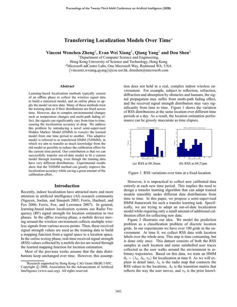
and the received signal strength distribution may vary significantly from time to time. Figure 1 shows the variation
of RSS distributions at the same location over different time
periods at a day. As a result, the location estimation performance can be grossly inaccurate as time elapses.
Learning-based localization methods typically consist
of an offline phase to collect the wireless signal data
to build a statistical model, and an online phase to apply the model on new data. Many of these methods treat
the training data as if their distributions are fixed across
time. However, due to complex environmental changes
such as temperature changes and multi-path fading effect, the signals can significantly vary from time to time,
causing the localization accuracy to drop. We address
this problem by introducing a novel semi-supervised
Hidden Markov Model (HMM) to transfer the learned
model from one time period to another. This adaptive
model is referred to as transferred HMM (TrHMM), in
which we aim to transfer as much knowledge from the
old model as possible to reduce the calibration effort for
the current time period. Our contribution is that we can
successfully transfer out-of-date model to fit a current
model through learning, even though the training data
have very different distributions. Experimental results
show that the TrHMM method can greatly improve the
localization accuracy while saving a great amount of the
calibration effort.
RSS from AP[00 0F 66 3A 1D 2A] at 04:21pm
14
12
12
10
10
Frequency
Frequency
RSS from AP[00 0F 66 3A 1D 2A] at 08:26am
14
8
6
4
6
4
2
0
8
2
−78
−76
−74
−72
−70
Signal strength (unit: dBm)
−68
(a) RSS at 08:26am
−66
0
−78
−76
−74
−72
−70
Signal strength (unit: dBm)
−68
−66
(b) RSS at 04:21pm
Figure 1: RSS variations over time at a fixed location.
However, it is impractical to collect new calibrated data
entirely at each new time period. This implies the need to
design a transfer learning algorithm that can adapt trained
models smoothly under different data distributions from
time to time. In this paper, we propose a semi-supervised
HMM framework for such a transfer learning task. Specifically, we are trying to adapt an out-of-date localization
model while requiring only a small amount of additional calibration effort for collecting new data.
Figure 2 illustrates our idea. We model the prediction
problem as a classification problem of discrete location
grids. In our experiments we have over 100 grids in the environment. At time 0, we collect RSS data with location
labels over the whole area. This step is time consuming, but
is done only once. This dataset consists of both the RSS
samples at each location and some unlabelled user traces
collected as the user walks around the environment in arbitrary trajectories. Based on this data, we train an HMM
θ0 = (λ0 , A0 , π0 ) for localization at time 0. As we will explain in detail later, λ0 is the radio map that connects the
RSS values to the locations, A0 is the transition matrix that
reflects the way the user moves, and π0 is the prior knowl-
Introduction
Recently, indoor localization have attracted more and more
attention in artificial intelligence (AI) research community
(Nguyen, Jordan, and Sinopoli 2005; Ferris, Haehnel, and
Fox 2006; Ferris, Fox, and Lawrence 2007). In general,
learning-based indoor localization systems use Radio Frequency (RF) signal strength for location estimation in two
phases. In the offline training phase, a mobile device moving around the wireless environment collects multiple wireless signals from various access points. Then, these received
signal strength values are used as the training data to build
a mapping function from a signal space to a location space.
In the online testing phase, real-time received signal strength
(RSS) values collected by a mobile device are tested through
the learned mapping function for location estimation.
Most of the previous works assume that the data distributions keep unchanged over time. However, this assump∗
Research supported by Hong Kong CAG Grant HKBU1/05C.
c 2008, Association for the Advancement of Artificial
Copyright Intelligence (www.aaai.org). All rights reserved.
1421
the new time periods. In the experimental section, we verify
our algorithm through some real-world data and show that,
compared with state-of-art methods, our TrHMM algorithm
can greatly improve the localization accuracy under different
data distributions while saving a large amount of calibration
efforts.
Related work
Generally, localization methods fall into two categories:
propagation-model based and machine-learning based.
Propagation-model based techniques rely on radio propagation models which use triangulation techniques for location
estimation (Savvides, Han, and Strivastava 2001). Learningbased techniques try to handle the uncertainty in wireless environments and use statistical learning such as KNN (Bahl
and Padmanabhan 2000), kernel learning (Nguyen, Jordan,
and Sinopoli 2005) and Gaussian process (Ferris, Haehnel,
and Fox 2006; Ferris, Fox, and Lawrence 2007). There are
few works on studying the data distribution variations in
wireless indoor localization. LANDMARC (Ni et al. 2003)
and LEASE (Krishnan et al. 2004) utilized a large number
of hardware equipments, including stationary emitters and
sniffers, to obtain up-to-date RSS values for updating the
radio maps. (Pan et al. 2007) used multi-view manifold
learning to constrain the agreements between different distributions. However, in practice, many of these works cannot
work well due to different model constraints.
Recently, there has been a growing interest in transfer
learning. Several researchers have explored specific aspects
of transfer learning in natural language and image processing areas (Thrun and Mitchell 1995; Ben-David and Schuller
2003). (DauméIII and Marcu 2006) investigated how to train
a general model with data from both a source domain and a
target domain for a natural language mention-type classification task. (Daumé III 2007) applied redundant copies of
features to facilitate the transfer of knowledge. In the area
of machine learning based localization, few work on transfer
learning has been done before.
Figure 2: Adapting a localization model from time 0 to time
t using TrHMM. The triangles denote reference point locations in the area.
edge on the likelihood of where the user is. Note that λ0 is
changing over time because signal strength varies. A0 can
also be changing over time because at different time periods,
people may have different activities. For example, at noon,
people are more likely to go to carteen for lunch; and during
working hours, people are more likely to move within the
office area. Therefore, both λ0 and A0 need to be adapted
to λt and At for a new time period t. π0 is kept unchanged
over time1 , since in reality, the basic human behavior does
not change dramatically. For example, a professor usually
stays at his office longer than his walking in a corridor.
In TrHMM, we carry out three steps for transferring with
respect to the three HMM model parameters (λ0 , A0 , π0 ):
• At time 0, we select some locations to place sniffing sensors to collect up-to-date RSS values. We call such set of
selected locations as ”reference points”. We then learn the
regression weights α among the RSS data from the few
reference points and the remaining non-reference points,
in order to transfer the radio map from time 0 to time t.
• We note that even though the data distributions change,
the relationship between neighboring locations do not
change much. This relationship can be used as a bridge
for transferring the knowledge over radio map change.
Therefore, by introducing a constraint that the regression
weights remain static, we build a radio map λt at each
non-reference point location at time t by collecting up-todate data on the few referent points (shown as Triangles
in Figure 2) with known locations.
Preliminaries of Hidden Markov Models
Hidden Markov Model is a well known technique in pattern
recognition and has a wide range of applications (Rabiner
1990; Bui, Venkatesh, and West 2002). In indoor localization, HMM can be used to model the user traces by treating
user’s locations as hidden states and the signal strength measurements as observations (Ladd et al. 2002). As shown in
Figure 3, an HMM for user-trace modeling is defined as a
quintuple (L, O, λ, A, π), where L is a location-state space
{l1 , l2 , ..., ln }, and each li is explained as a discrete grid cell
of the physical locations with x− and y− coordinates: li =
(xi , yi ). O is an observation space {o1 , o2 , ..., om }, and
each oj is a set of k signal strength measurements received
from k different Access Points (APs): oj = (s1 , s2 , ..., sk ).
λ is a radio map {P (oj |li ) : oj ∈ O, li ∈ L} that gives the
conditional probability of obtaining a signal strength measurement oj at location li . A is a location-state transition
matrix {P (lj |li ) : li , lj ∈ L}; it encodes the probability for
a user moving from one location li to another location lj . π
• At time t, some unlabeled user traces are collected by simply walking around the environment. Since these traces
data encode the knowledge of current time period data
distribution and also the user transition behaviors, they
are further used to transfer the localization model to λnew
t
and At by an expectation-maximization (EM) algorithm.
Note that our choice of using HMM model is motivated
by the following considerations. Compared with other localization models, HMM can utilize both single RSS samples
and user trajectories in the form of sequential knowledge.
Therefore, we may be able to transfer more information for
1
However, a changing π0 can be addressed in an extension of
this work.
1422
is an initial location-state distribution {P (li ), li ∈ L} with
each P (li ) encoding the prior knowledge about where a user
initially may be.
P(l1)
P(l1|l2)
l1
P(l 2|l3)
l2
P(o1|l1)
O1
time, the signal on its neighboring location l2 is also likely
to increase. Motivated by this observation, we apply a regression model to learn the temporal predictive correlations
between the RSS values by sparsely located reference points
and that by the mobile device. Specifically, we apply a Multiple Linear Regression model on the data at time 0 over
all the location grids, and derive the regression coefficients
αk = {αkij }, which encode the signal correlations between
reference point locations {lc } and one non-reference point
location k. In more detail, we have:
l3
...
P(o2|l2)
O2
lt
O3
...
Ot
skj = αk0j + αk1j r1j + ... + αknj rnj + ǫj
(2)
where skj is the signal strength received by the mobile device
at location k from j th AP, αkij : 1 ≤ i ≤ n is the regression
weights for j th AP signal at location k, and rij : 1 ≤ i ≤ n
is the signal strength received by ith reference point location
from j th AP.
Figure 3: Hidden Markov Model.
In the offline training phase, a set of labeled traces T =
{(tri , qi ) : i = 1, ..., N } is collected, with each user trace
tri = (o1 , o2 , ..., o|t| ) and the corresponding location sequence qi = (l1 , l2 , ..., l|t| ). Here, oj ∈ O and lj ∈ L.
Then, these labeled traces are used to train an HMM. We
denote an HMM’s parameters as θ = (λ, A, π). The radio
map λ can be obtained by modeling the conditional probability P (oj |li ) as a Gaussian distribution:
T
1
1
P (oj |li ) =
e− 2 (oj −µ) Σ(oj −µ) , (1)
(2π)k/2 |Σ|1/2
where µ is the mean vector of the observations, and Σ is the
covariance matrix. By assuming the independence among
the APs (Ladd et al. 2002), we can simplify Σ as a diagonal
matrix. The transition matrix A = {P (li+1 |li )} encodes the
probability for a mobile device to move from one location li
to another location li+1 . It can be easily obtained from the
labeled traces by counting the transition statistics of each
location to all possible next locations. In an indoor environment, a mobile device carried by a human being usually does
not move too fast, which allows us to constrain the transition
probability P (li+1 |li ) to be zero if li+1 is more than a few
meters away from li ; in our experiments we set the threshold as three meters. The initial location-state distribution π
can be derived by our prior knowledge. Generally, it is set
by a uniform distribution over all the locations, since a user
can start at will from any location. This assumption can be
revised easily if we have more prior knowledge about user
location patterns.
In the online test phase, given a model parameter θ and an
observed user trace tr = (o1 , o2 , ..., o|tr| ), the well-known
Viterbi algorithm (Rabiner 1990) can then be used to infer
the most probable hidden state sequence q.
Rebuilding the radio map at time t
After learning the regression weight αk for each nonreference point location k, we can use them to rebuild the
radio map at time t. This is done by updating non-reference
point locations’ signal strengths with the newly collected
signal strengths on the reference point locations {lc }, whose
locations are known beforehand. Considering that there may
be a possible shift for the regression parameters over time,
we add a tradeoff constraint to derive the new λt :
µt = β · µ0 + (1 − β) · µreg
t
h
i
T
Σt = β · Σ0 + (µt − µ0 ) (µt − µ0 )
h
i
reg T
+(1 − β) · Σreg
+ (µt − µreg
t
t ) (µt − µt )
(3)
(4)
where µ is the mean vector of Gaussian output for each
location, Σ is the covariance matrix. We balance the rereg
= (µreg
gressed radio map λreg
t , Σt ) and the base radio
t
map λ0 = (µ0 , Σ0 ) by introducing a parameter β ∈ [0, 1].
Using EM on unlabeled traces at time t
In previous steps, we first trained an HMM θ0 =
(λ0 , A0 , π0 ) at time 0 as the base model. Then, in another
time t, we improve λ0 by applying the regression analysis,
and obtain a new HMM θt = (λt , A0 , π0 ). Now we will try
to further incorporate some unlabeled trace data to improve
the derived θt . We achieve this by applying the expectationmaximization (EM) algorithm.
Given a set of unlabeled traces T = {(tri , qi )} , EM is
used to adjust the model parameters θt = (λt , A0 , π0 ) iteratively to find a θ∗ such that the likelihood P (T |θ∗ ) is
maximized. Recall that here tri is a sequence of RSS observations on a trace i, and qi are its corresponding locations.
Therefore, maximizing the likelihood P (T |θ∗ ) is to adapt
the model θt to best fit the up-to-date unlabeled traces data.
By using such adaptation, the HMM can be more accurate
in location estimation for the new time period t’s data. The
EM algorithm has two steps in each iteration: an Expectation step (E-step) and a Maximization step (M-step). For
TrHMM: Transferred Hidden Markov Model
As mentioned above, we use three steps to transfer the HMM
for the new time period.
Applying regression analysis at time 0
Our first step is to transfer the collected radio map λ0 at
time 0 to another time t. To do this, we propose to model
the signal variation with time. Note that in a wireless indoor environment, signals over different locations are correlated, e.g., when the signal on a location l1 increases with
1423
Algorithm 1 Transferred Hidden Markov Model (TrHMM)
Input: Labeled traces at time 0, labeled RSS samples collected from reference points and unlabeled traces at time t
Output: Adapted model θtnew = (λnew
, Anew
, π0 )
t
t
At time 0,
the k-iteration, in E-step, we calculate the conditional probability P (q|tr, θk ), i.e. location estimations q given the RSS
observations tr, from the unlabeled trace data T by using
the θk from last iteration’s M-step:
P (tr, q|θk )
P (tr|q, θk )P (q|θk )
P
P (q|tr, θk ) =
=
k
k
P (tr|θk )
q P (tr|q, θ )P (q|θ )
(5)
Q|tr|
where P (tr|q, θk ) = n=1 P (on |ln , θk ) is the likelihood
of observing a trace tr given the mobile device’s location
sequence is q. Notice that this term can be calculated from
the last M-step k’s radio map λk , since λk already encodes the conditional probability of P (on |ln ). The term
Q|tr|
P (q|θk ) = P (l1 |θk ) × n=1 P (ln |ln−1 , θk ) is the probability of q being location sequence in a user trace. This
can be calculated from prior knowledge π0 and transition
matrix Ak , because π0 encodes the probabilities of P (ln )
and Ak encodes the conditional probabilities P (ln |ln−1 ) for
different n’s. In the M-step, an expected loglikelihood (i.e.
Q-function) is maximized over the parameter θ based on the
E-step. The parameter θk is then updated to obtain θk+1 :
θk+1 = arg max Q(θ, θk )
θ
P P
= arg max
P (q|tr, θk ) log P (tr, q|θ)
θ
1. Build an HMM base model θ0 = (λ0 , A0 , π0 ) using labeled traces from time 0;
2. Learn the signal regression weights αk among referent
points and the rest, using labeled trace data from time 0;
At time t,
1. Rebuild the radio map using the labeled RSS samples
collected from reference points at time t, and update the
model to θt = (λt , A0 , π0 );
2. Apply EM to improve θt as θtnew = (λnew
, Anew
, π0 ), by
t
t
using unlabeled traces from time t;
3. Return the HMM model θtnew = (λnew
, Anew
, π0 ).
t
t
(6)
tr∈T q
In particular, by following the derivation of (Bilmes
1997), we show the update for each parameter in θk+1 =
(λk+1 , Ak+1 , π). Note that since π is the prior knowledge
of the user locations, it’s set to be fixed and not involved in
EM. Specifically, the radio map λk+1 = {P (oj |li )(k+1) :
oj ∈ O, li ∈ L} is shown to be updated by:
P
P|tr| n
n
k
(k+1)
tr∈T
n=1 o P (l = li |tr, θ )
µ li
= P
P|tr|
n
k
tr∈T
n=1 P (l = li |tr, θ )
(k+1)
Σl i
=
P |tr|
P
tr∈T n=1
(on − µli )(on − µli )T P (ln = li |tr, θk )
P
tr∈T
P|tr|
n=1
P (ln = li |tr, θk )
(7)
And the transition matrix Ak+1 = {P (lj |li )(k+1) :
li , lj ∈ L} is updated as:
P
P|tr|−1
n
n+1
= lj |tr, θk )
tr∈T
n=1 P (l = li , l
(k+1)
P (lj |li )
=
P
P|tr|−1
n
k
tr∈T
n=1 P (l = li |tr, θ )
(8)
The EM algorithm guarantees the likelihood
P (T |θk+1 ) ≥ P (T |θk ) and the parameter θ eventually converges to a stable θ∗ . The new HMM is finally
updated as θtnew = (λnew
, Anew
, π0 ). In the online phase at
t
t
time t, the derived parameters in θtnew are used to infer the
most probable location sequence for the queried trace based
on Viterbi algorithm (Bilmes 1997), given the obtained RSS
values. We summarize our TrHMM in Algorithm 1.
Experiments
802.11g wireless network. The area is 64m × 50m, including five hallways. It’s discretized into a space of 118 grids,
each measuring 1.5m × 1.5m. Our experimental evaluation
method is based on classification accuracy, which is calculated as the percentage of correct predictions over all predictions. The problem is difficult because a random guess
would result in less than 1% in accuracy.
We collected calibration data over three time periods:
08:26am, 04:21pm and 07:10pm. We use 08:26am data to
build the base model and carry out adaptation on other time
periods. 60 samples were collected at each grid. We randomly splitted 2/3 of the data as training and 1/3 as testing.
Traces for building HMM were also collected at each time
period. For training, we have 30 labeled traces for 08:26am
data, each having 20 samples on average. In the remaining time periods, we obtained 30 unlabeled traces, each having 250 samples for training. For testing, we have 20 traces
for each time period, each having 250 samples on average.
In the experiments, β is set as 0.4. We tested different βvalues2 , and found that for different time periods, the performances with different β-values are similar, and β = 0.4
gives roughly the best results. This coincides with our intuition of allocating around half the weight to the regressed
radio map and old radio map in Equation (3).
Impact of distribution variation
We test the localization accuracy over different data distributions without adaptation. We use the 08:26am dataset to
build the base model θ0 , and then apply θ0 to predict the labels for test data traces of the three time periods. We use
10% of locations as reference points and 5 unlabeled traces
for adaptation. As shown in Figure 4, the localization accuracy of 08:26am data is the highest, at 92%3 . This high
2
We do not provide the results here due to space limit.
The error distance is set to be 3 meters, which means the predictions within 3 meters of the true location are all counted as correct predictions.
In this section, we empirically study the benefits of transferring HMM for adapting indoor localization. Our experiments were set up in an academic building equipped with
3
1424
accuracy is due to the fact that the test data follow the same
distribution with the training data. As time goes by, the
signals become more noisy and changing, and the performance drops. At 04:21pm, the busiest time in the work area,
the noise level reaches the highest because of many people
walking around at that time. During this period, the accuracy thus drops to the lowest point to about 68%, which is
unsatisfactory. This observation implies a need for transferring the localization model over different data distributions.
(UnHMM) (Chai and Yang 2005), which only uses unlabeled traces. UnHMM builds a base model θ0 , and then
directly use EM to iteratively update the model θ0 using
the unlabeled traces. The second method is LeManCoR,
which uses unlabeled data for manifold regularization in
adaptation. We use 10% of locations as reference points for
both TrHMM and LeManCoR. We run the experiments for
5 times and report the error bar chart. As shown in Figures 5(c) and 5(d), our TrHMM consistently outperforms
the baselines. Our TrHMM can outperform UnHMM because TrHMM carefully models the signal variation over
time while UnHMM not. Our method also outperforms LeManCoR because TrHMM better models the signal variations and also uses the sequential information in traces.
1
0.95
Culmulative probability
0.9
0.85
Sensitivity to error distance
0.8
We study the sensitivity of TrHMM to different error distances. In experiment, 10% locations were used as reference
points for collecting labeled data and 5 traces were used for
unlabeled data. We run the experiments for 5 times and
report the error bar charts. As shown in Figures 5(e) and
5(f), our TrHMM method is insensitive to the error distance
in calculating the localization accuracy4. In addition, compared to other localization methods, our TrHMM can work
much better even when the error distance is small. Both of
these observations testifies our TrHMM method can provide
accurate location estimation with small calibration effort.
0.75
0.7
0.65
0.6
08:26am
04:21pm
Time periods
07:10pm
Figure 4: Use 08:26am model to predict others.
Impact of reference points
We next study the impact of using different number of reference points, i.e. different amount of labeled data, for adaptation. We compare TrHMM with three baselines using reference points for adaptation, including RADAR (Bahl and
Padmanabhan 2000), LANDMARC (Ni et al. 2003) and
an recent adaptation method, LeManCoR (Pan et al. 2007).
RADAR is a K-nearest-neighbor method. The number of
nearest neighbors is set to be five, as tested in (Bahl and
Padmanabhan 2000). LANDMARC is a nearest-neighbor
weighting based method. In this experiment, the number
of nearest neighbors is set to two, since only few reference
points are sparsely deployed in the environment. LeManCoR is a semi-supervised manifold method. It treats different time as multiple views and uses a multi-view learning
framework to constraint the predictions on reference points
to be consistent. In this experiment, we use 5 unlabeled
traces for both TrHMM and LeManCoR. We run the experiments for 5 times and report the error bar charts. As
shown in Figures 5(a) and 5(b), our TrHMM consistently
outperforms the other methods over time, especially when
the number of reference points is small. For RADAR and
LANDMARC, they can only work when the environment
is densely installed with reference points. For LeManCoR,
as discussed in (Pan et al. 2007), it cannot benefit from either the increasing number of reference points or the trace
sequential information, so our TrHMM method can outperform it consistently.
Conclusions and Future Work
In this paper, we study the problem of transfer learning using a semi-supervised HMM for adaptive localization in a
dynamic indoor environment. We carefully model the signal variation with time and employ a semi-supervised HMM
framework, which appropriately combine both labeled data
and unlabeled data together for model adaptation. By applying it to the real-world indoor localization, we show our
TrHMM algorithm can greatly improve the accuracy while
saving a great amount of the calibration efforts, even when
the data distribution is a function of time. Our experiments
confirm that our TrHMM can successfully transfer the outof-date model to current time periods.
In the future, we plan to extend this algorithm to online
setting such that the system can make predictions while it
collects new trace data. Besides, we would consider how to
optimally place the reference points for adaptation. We are
also interested in incorporating transfer learning with Gaussian process for localization.
References
Bahl, P., and Padmanabhan, V. N. 2000. RADAR: An inbuilding RF-based user location and tracking system. In
INFOCOM (2), 775–784.
Ben-David, S., and Schuller, R. 2003. Exploiting task relatedness for multiple task learning. In Proceedings of the Sixteenth Annual Conference on Learning Theory, 825–830.
Impact of unlabeled data
We also study the impact of using different number of unlabeled traces for adaptation. We compare TrHMM with two
baseline methods. The first method is unsupervised HMM
4
Note that the predictions of HMM are discrete hidden variables, which in our case are 1.5m × 1.5m grids, so the accuracy is
stable from 1.75m to 3m.
1425
04:21pm
07:10pm
1
1
0.9
0.9
0.8
0.8
04:21pm
0.9
0.7
0.6
0.5
TrHMM
LeManCoR
RADAR
LANDMARC
0.4
10%
20%
Culmulative probability
Culmulative probability
Culmulative probability
0.85
0.7
0.6
0.5
30% 40% 50% 60% 70% 80% 90%
Ratio of locations used for reference points
10%
20%
0.7
0.65
0
30% 40% 50% 60% 70% 80% 90%
Ratio of locations used for reference points
(a) Impact of reference points for 04:21pm (b) Impact of reference points for 07:10pm
07:10pm
0.8
0.75
10
15
20
Number of unlabled traces
25
0.9
0.8
0.8
0.7
0.7
0.6
0.5
0.4
0.3
(d) Impact of unlabeled data for 07:10pm
0
1.5
1.75
2
30
2.25
2.5
Error distance (m)
2.75
0.6
0.5
0.4
0.3
0.2
TrHMM
LeManCoR
RADAR
LANDMARC
0.1
30
25
07:10pm
0.9
0.2
TrHMM
UnHMM
LeManCoR
5
10
15
20
Number of unlabled traces
(c) Impact of unlabeled data for 04:21pm
Culmulative probability
Culmulative probability
Culmulative probability
0.85
0.65
0
5
04:21pm
0.9
0.7
0.75
TrHMM
LeManCoR
RADAR
LANDMARC
0.4
TrHMM
UnHMM
LeManCoR
0.8
TrHMM
LeManCoR
RADAR
LANDMARC
0.1
3
0
1.5
1.75
2
2.25
2.5
Error distance (m)
2.75
3
(e) Sensitivity to error distance for 04:21pm (f) Sensitivity to error distance for 07:10pm
Figure 5: Experimental results
Bilmes, J. 1997. A gentle tutorial on the em algorithm and
its application to parameter estimation for gaussian mixture
and hidden markov models. In Technical Report, University of Berkeley, ICSI-TR-97-021, 1997.
Bui, H.; Venkatesh, S.; and West, G. 2002. Policy recognition in the abstract hidden markov models. Journal of
Artificial Intelligence Research 17:451–499.
Chai, X., and Yang, Q. 2005. Reducing the calibration
effort for location estimation using unlabeled samples. In
IEEE PerCom’05, 95–104.
Daumé III, H. 2007. Frustratingly easy domain adaptation. In Conference of the Association for Computational
Linguistics (ACL).
DauméIII, H., and Marcu, D. 2006. Domain adaptation
for statistical classifiers. Journal of Artificial Intelligence
Research 26:101–126.
Ferris, B.; Fox, D.; and Lawrence, N. 2007. Wifi-slam
using gaussian process latent variable models. In International Joint Conferences on Artificial Intelligence, 2480–
2485.
Ferris, B.; Haehnel, D.; and Fox, D. 2006. Gaussian
processes for signal strength-based location estimation. In
Proceedings of Robotics: Science and Systems.
Krishnan, P.; Krishnakumar, A. S.; Ju, W.-H.; Mallows, C.;
and Ganu, S. 2004. A system for lease: Location estimation assisted by stationery emitters for indoor rf wireless
networks. In INFOCOM’04.
Ladd, A. M.; Bekris, K. E.; Rudys, A.; Kavraki, L. E.; Wal-
lach, D. S.; and Marceau, G. 2002. Robotics-based location
sensing using wireless ethernet. In Proceedings of the 8th
annual international conference on Mobile computing and
networking, 227–238.
Nguyen, X.; Jordan, M. I.; and Sinopoli, B. 2005. A
kernel-based learning approach to ad hoc sensor network
localization. ACM Trans. Sen. Netw. 1(1):134–152.
Ni, L. M.; Liu, Y.; Lau, Y. C.; and Patil, A. P. 2003. Landmarc: indoor location sensing using active rfid. In IEEE
PerCom’03.
Pan, S. J.; Kwok, J. T.; Yang, Q.; and Pan, J. J. 2007. Adaptive localization in a dynamic wifi environment through
multi-view learning. In Proceedings of the Twenty-Second
National Conference on Artificial Intelligence, 1108–1113.
Rabiner, L. R. 1990. A tutorial on hidden markov models
and selected applications in speech recognition. In Readings in speech recognition. San Francisco, CA, USA: Morgan Kaufmann Publishers Inc. 267–296.
Savvides, A.; Han, C.-C.; and Strivastava, M. B. 2001. Dynamic fine-grained localization in ad-hoc networks of sensors. In MobiCom ’01: Proceedings of the 7th annual international conference on Mobile computing and networking,
166–179. New York, NY, USA: ACM.
Thrun, S., and Mitchell, T. M. 1995. Learning one more
thing. In Proceedings of the Fourteenth International Joint
Conference on Artificial Intelligence, 825–830.
1426