Quasi-Monotonic Segmentation of State Variable Behavior for Reactive Control
Will Fitzgerald
Daniel Lemire
Martin Brooks
QSS Group, Inc.
NASA Ames Research Center
Moffett Field, CA, 94035
University of Quebec in Montreal
4750 Henri-Julien
Montréal, QC H2T 3E4
National Research Council of Canada
1200 Montreal Road
Ottawa, ON K1A 0R6
Abstract
Real-world agents must react to changing conditions as they
execute planned tasks. Conditions are typically monitored
through time series representing state variables. While some
predicates on these times series only consider one measure
at a time, other predicates, sometimes called episodic predicates, consider sets of measures. We consider a special class
of episodic predicates based on segmentation of the the measures into quasi-monotonic intervals where each interval is either quasi-increasing, quasi-decreasing, or quasi-flat. While
being scale-based, this approach is also computational efficient and results can be computed exactly without need for
approximation algorithms. Our approach is compared to linear spline and regression analysis.
Reactive control and monitoring
It has been recognized for some time that real-world agents
have to monitor conditions as they execute planned tasks.
It is rarely the case that the only changes that can occur in
the world result from actions taken by the agent. Actions
taken by other agents, uncontrollable events occurring in the
physical world, and the presence of noise and uncertainty
are the norm.
Given this, an agent must be able to react to changes in
the world. Moreover, the agent must be able to notice the
changes in the first place. A typical description of this is a
three-tiered architecture (Bonasso et al. 1997), with sensors
and effectors at the “bottom” tier, and a high-level planner at
the “top” tier. In between, the task execution system monitors for changing conditions and executes actions as appropriate based on the goals given it by the planner. Reactive
task execution systems include EXEC (Pell et al. 1997), the
RAP System (Firby 1989), PRS (Myers 1996), and Apex
(Freed et al. 2003).
Of course, the conditions to which an agent might imaginably react can be arbitrarily complex, and, for an agent
acting in the real world, a “paralysis of analysis” prevents
effective action. Part of an effective architecture for agent
design is describing the kinds of useful conditions which are
likely to be relevant to the agent making use of the kinds of
sensors typically available to the agent. Furthermore, it must
be feasible–that is, computational efficient–to recognize the
c 2005, American Association for Artificial IntelliCopyright gence (www.aaai.org). All rights reserved.
relevant conditions, especially in concert with a variety of
simultaneously executing tasks and monitors.
Sensors nominally create time-stamped data, with readings sometimes done at constant intervals, sometimes not.
Each reading provides a time-stamped measurement of a
state variable, that is, an attribute of some object (often
the agent, or a component of the agent), which changes
over time. For example, an autonomous aircraft will typically have sensors for its own altitude, longitude and latitude, among other measurements. Tasks such as “raise-gear”
might have a precondition that the measured altitude be ≥ a
certain amount.
Given the time series nature of such sensor data, it is natural to consider monitors being “live” for some interval of
time. Within such an interval I, we have an ordered set of
measurements for a given sensor, {xt }, ordered by time t.
If P is a boolean predicate on x, and n is the cardinality
of {xt }, then testing for a value in I upon which P is true
is clearly at least O(n). In a typical case, P is of constant
complexity (such as the example of ≥ given above), and so,
testing for value upon which P is true is O(n).
Predicates on individual measurement values are not the
only possible boolean predicates of interest. For example,
an agent might want to act when the average value of a measurement within an interval reaches a certain point. The
presence of a condition based on multiple measurements (of
the same or different state variable) is sometimes called an
episode (Mannila, Toivonen, & Verkamo 1997). Episodic
predicates can, of course, be arbitrarily complex, and thus be
difficult or impossible for an agent to consider. In this paper, we discuss one particular class of episodic predicates,
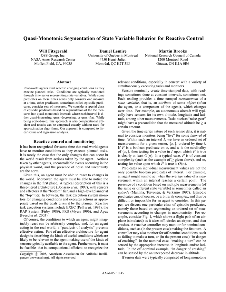
namely those based on segmenting an ordered set of measurements according to changes in monotonicity. For example, consider Fig. 1, which shows a flight path of an airplane (simulated) as it takes off, circles an airport, and then
crashes. A reactive controller may monitor for nominal conditions, such as (in the present case) making the first turn. A
controller may also monitor for off-nominal conditions, such
as failing to make a turn, or (in the present case) “in danger
of crashing.” In the nominal case, “making a turn” can be
sensed by the appropriate increase in longitude and/or latitude. In the off-nominal example, “in danger of crashing”
can be sensed by the an unexpected decrease in altitude.
If sensor data were typically comprised of long monotone
AAAI-05 / 1145
11
10
9
1400
8
1200
7
1000
800
6
600
5
400
200
4
0
3
10.5
10.4
Figure 1: Flight path of airplane
10.3
10.2
segments, then such a change in monotonicity would be trivial to detect. Sensors, of course, do not do so, for a variety
of reasons. First, sensors are typically sampled at some rate,
creating discontinuities. Second, exogenous events cause
changes in sensor values which can be non-continuous; indeed, if this were not the case, there would be little need for
sensors. Third, sensors inherently produce some amount of
error, which can be minimized but never eliminated.
Consider the two plots in Fig. 2, which show real data
from a life-support application, showing the measured mass
of a distillant in a tank. The top plot exemplifies “noise” due
to exogenous events. It is clear that the mass increases (as
distillant flows into the tank), then decreases (as it is pumped
out of the tank). There are slight “jags” on the increase and
decrease (due to some exogenous event such as a cycling
pump), but these can be ignored. There is another indication
of noise at the beginning of the first increase, probably due
to someone picking up the tank and replacing it.
The second plot exemplifies the other kinds of noise; this
magnification of the first peak shows the discrete nature of
sampling and the inherent error of the scale become evident.
Essentially, we would like to segment the time series of
measurements of a state variable into regions of alternating
sign, ignoring small violations of monotonicity. An algorithm for doing this has three desiderata: (1) it must provide such a segmentation in a way that is both intuitively
and mathematically sound; (2) it must be computationally
efficient enough to run in real time, and (3) ideally, it is an
on-line algorithm that can be updated efficiently as an agent
acts and senses in the world.
In this paper, we present an algorithm for segmentation of state variable measurements based on the quasimonotonic segmentation ideas of (Brooks 1994), which provides a mathematically well-motivated notion of monotonic
segmentation at a given scale. The algorithm is O(n), where
n in the number of measurements, and only requires constant space. It is also an on-line algorithm, whose update
runs in constant time and space. We contrast this with algorithms typically used for segmentation, based on linear
splining and regression techniques, which provide less intuitive results and are, in fact, O(n2 ).
10.1
10
9.9
9.8
Figure 2: Mass data at different scales
Quasi-monotonic segmentation
For a state variable x, say that an ordered set of measurements of x, {xk } is monotonic if either xk ≥ xk+1 or
xk ≤ xk+1 . As we have stated, this does not capture an interesting understanding of “monotonic,” due to the sources
of noise mentioned above. For practical applications, we
want to tolerate some deviation from monotonicity. One
possible way to describe allowing such a toleration is to say,
given an ordered set of measurements {xk } and some tolerance value δ > 0, that the data points are not going down
or are upward monotone, if consecutive measures do not go
down by more than δ, that is, are such that xi − xi+1 > δ.
However, this definition is not very useful because measures
can repeatedly go down and (eventually) the end value can
be substantially lower than the start value. A more useful
definition of upward monotonicity is to require that we cannot find two successive measures xi and xj (j > i) such
that xj is lower than xi by δ (xi − xj > δ). This definition
is more useful because in the worse case, the last measure
will be only δ smaller than the first measure. However, we
are still not guaranteed that the data does in fact increase.
Hence, we ask that we can find at least two successive measures xk and xl (l > k) such that xl is greater than xk by at
least δ (xl − xk ≥ δ).
In order to formalize this concept, we will use the idea of
δ-pair introduced in (Brooks 1994) (see Fig. 3). Let F be a
function, and D be its domain. The tuple x, y (x < y ∈ D)
is a δ-pair (or a pair of scale δ) for F if |F (y) − F (x)| ≥ δ
and for all z ∈ D, x < z < y implies |F (z) − F (x)| < δ
and |F (y) − F (z)| < δ. A δ-pair’s direction is increasing or
AAAI-05 / 1146
δ
δ
δ −pair
Figure 3: A δ-pair.
decreasing according to whether F (y) > F (x) or F (y) <
F (x).
Notice that pairs of scale δ having opposite directions cannot overlap but they may share an end point. Pairs of scale
δ of the same direction may overlap, but may not be nested.
We use the term “pair” to indicate a δ-pair having an unspecified δ.
We say that a sequence of measures X = {xk }k is δmonotonic if all δ-pairs have the same sign (all increasing or
all decreasing). Given a δ-monotonic data set, we say that it
is δ-flat if it contains no δ-pair and it is δ-increasing (resp.
decreasing) if all δ-pairs are increasing (resp. decreasing).
Given a sequence of measures X = {xk }k=1,...,N , a segmentation X1 . . . Xn is given by a set of n + 1 indices yi
such that yi+1 > yi , y1 = 1 and yn+1 = N and where
Xi = {xk }k=yi ,...,yi+1 . A segmentation is an extremal segmentation at scale δ if
1. All Xi are δ-monotone;
2. No two adjacent segments have the same monotonicity
(flat, increasing, decreasing);
3. For i = 2, . . . , n, xyi = max Xi ∪ Xi−1 or xyi =
min Xi ∪ Xi−1 ;
4. Unless X1 is δ-flat, x1 = max X1 or x1 = min X1 ;
unless Xn is δ-flat, xN = max Xn or xN = min Xn .
The merger of a δ-increasing (resp. decreasing) segment with a δ-flat segment is δ-increasing (resp. decreasing). Hence, depending on whether or not we consider δ-flat
segments, we can have various extremal segmentation with
varying number of segments. However, if we exclude δ-flat
segments, then the number of segments will be the same for
all extremal segmentations at the same scale.
Algorithm for segmentation
Algorithm 1 presents an algorithm for quasi-monotone segmentation. A queue is initialized with the index of the first
measurement. After determining the initial direction of the
measurements, it scans through the measurements, keeping
a back-pointer to the last extremum, which is initialized to
the first position. When the difference between an element
and the measurement at the back-pointer exceeds δ, and the
new δ-pair switches signs, a new extremum is added to the
queue, the sign is flipped and the back-pointer updated. After completing the scan, the index of the last measurement is
added to the queue if it isn’t already present.
Basic initialization (lines 4–6) take constant time. The
determineSign function takes no more than n − 1 steps (in
practice, it will take many fewer). The algorithm is dominated by the loop in lines 8–19, which is run n times. All of
the comparisons and assignments within the loop take constant time; thus the loop runs in O(n). Checking for the
presence of the last index in the queue (line 20), and adding
it to the queue if it isn’t present, takes constant time. Thus,
Algorithm 1 is O(n).
All variables (except for the output queue) in Algorithm 1
take constant space.
Note that Algorithm 1 can easily be converted to an online algorithm by converting the for loop into a stream consumer. As new measurements arrive, they either result in a
new extremum, in which case the new extremum is output.
Theorem 1 Algorithm 1 generates an extremal segmentation at scale δ.
Proof. Any segment having last index k that was added to
Q while D = 1 cannot have decreasing δ-pairs. Indeed,
suppose that there exist indexes l, j in the segment such that
l < j and xl − xj ≥ δ. When i (the variable of the main
for loop) took value j, the maximum of the segment up to
this point was xk with xk ≥ xl ⇒ xk − xj ≥ xl − xj and
because j is included in the segment, xk − xj < δ hence
xl − xj δ.Similarly, we could also show that segments with
D = −1 cannot have increasing δ-pairs.
Next, notice that the end of all segments, except possible the last two, is set before or at the beginning of a δpair with an opposite direction (decreasing if D = 1 or vice
versa). This means that all segments except possibly the first
one and the last one are either δ-increasing or δ-decreasing
and they alternate. Observe that when either of the first or
last segment is neither δ-increasing nor δ-decreasing, then it
must be δ-flat.
As the next theorem shows, our definitions and Algorithm 1 allow for a multiscale analysis: we can relate analyses done at different scales. In short, as we reduce the tolerance, existing segments will be partitioned and new endpoints will be added, but existing end-points will remain.
Theorem 2 Using Algorithm 1, the segmentation points
found with δ 0 < δ include those found with δ.
Proof. At scale δ and as per Algorithm 1, consider an increasing segment ending at index j 0 followed by a decreasing segment. We have that xj 0 is the maximum of both segments. A pair at scale δ, must contain a pair at scale δ 0 for all
δ 0 < δ. Hence, a segment increasing (decreasing) at scale δ
must contain a segment increasing (resp. decreasing) a scale
δ 0 . Hence, there is at least one pair at scale δ 0 before (and
after) j 0 . Consider the last pair at scale δ 0 before j 0 , we see
that it must be an increasing pair because xj 0 is a maximum:
if the last pair is decreasing, then its starting point would
have a value greater than xj 0 which is impossible. Similarly,
the first pair at scale δ 0 after j 0 is decreasing. Because j 0
is the index of the first maximum with value xj 0 before the
first pair, it will be selected by the algorithm at scale δ 0 . By
symmetry, the same result is shown for a segmentation point
following a decreasing segment.
AAAI-05 / 1147
Consider now the second segmentation point (at index j)
preceded by a flat segment and followed by a decreasing
segment at scale δ. We have that xj is the maximum of
both segments. The first pair at scale δ 0 following j must be
decreasing and the last pair before j at scale δ 0 , if it exists,
must be increasing. Hence, j must be a segmentation point
at scale δ 0 . The result is shown similarly when j is the index
of a minimum or the second last segmentation point at scale
δ.
Algorithm 1 Algorithm for quasi-monotone segmentation.
1: INPUT: sequence of values xi with i = 1, . . . , n
2: INPUT: scale δ
3: OUTPUT: an ordered sequence of indices which define
the segmentation
4: Q ← empty queue
5: place 1 in Q
6: k ← 1
7: D ← determineSign(x)
8: if D = 0 then
9:
add n to Q
10:
exit with Q
11: for i ∈ {1, . . . , n − 1} do
12:
if (D = 1 and xk −xi ≥ δ) or (D = −1 and xi −xk ≥
δ) then
13:
add k to Q
14:
flip sign of D
15:
else if (D = 1 and xi > xk ) or (D = −1 and xi <
xk ) then
16:
k←i
17: if last(Q) isn’t k and size(Q)>1 then
18:
add k to Q
19: if last(Q) isn’t n then
20:
add n to Q
21: exit with Q
1: FUNCTION determineSign
2: INPUT: sequence of values xi with i = 1, . . . , n
3: OUTPUT: initial direction as -1,1 or 0
4: for i in {2, n} do
5:
if xi 6= x0 then
6:
exit with sign of xi − x0
7: exit with 0
1
0.8
0.6
0.4
0.2
0
1
0.8
0.6
0.4
0.2
0
Figure 4: Segmented latitude and longitude data.
The mass of the tank plus distillant plotted in Fig. 6 ranges
from about 5 to 11 (except for the anomalous drop to 4).
With δ set to 1, the data are placed into six segments: one
ending at the anomalous drop, the other five tracking the
general rise and fall of the sensed mass.
Comparison to other methods
Segmenting data is a standard problem in time series research; a useful survey can be found in (Keogh et al. 1993),
who identify three types of approaches: sliding windows, in
which a segment is grown until an error bound is reached;
top-down, in which a time-series is recursively partitioned,
and bottom-up, in which larger and larger segments are
merged, starting from smallest segments. Keogh et al. also
Examples
1
Figures 4, 5, and 6 show the results of running Algorithm 1
on the aircraft data and mass data described above. The three
state variables of the aircraft data (latitude, longitude, and
altitude) are plotted separately, and normalized to 1.01 . The
longitude and latitude data have been split into three segments, with the middle segment beginning and ending where
the aircraft began its two turns. The altitude data has been
split into two segments: its steep then gradual rise, and its
steep decline (and crash).
0.8
0.6
0.4
0.2
0
1
In the simulation, the aircraft did not fly very far–no more than
20 kilometers in either direction–so no conversion from angular
measurements have been made here.
AAAI-05 / 1148
Figure 5: Segmented altitude data.
11
Quasi-monotone
Sliding Window
Least squares fit: ax2+bxc
20000
10
9
15000
8
7
10000
6
5
5000
4
3
0
0
Figure 6: Segmented mass data.
5000
10000
15000
20000
25000
30000
35000
40000
Figure 8: Execution time: Alg.1 versus Sliding Window.
Note the execution time of Alg. 1 is close to the zero axis.
0.08
0.06
0.04
0.02
0
-0.02
-0.04
-0.06
-0.08
-0.1
Figure 7: Damped sign wave with noise
provide an algorithm, SWAB, which combines a sliding
window and bottom-up approach (SWAB stands for “sliding window and bottom-up”).
Keogh et al.’s complexity analysis reveals that the topdown algorithms have a complexity of O(n2 K), where K
is the number of segments created, and n is the number of
points in the time series. The sliding window, bottom-up,
and SWAB algorithms have a complexity of O(n2 /K).
It is interesting to consider what happens as more or fewer
segments are created. The maximum number of segments is
n − 1, resulting when each point is paired with its successor
to create a segment, up to n − 1. In this case, the complexity
of top-down in O(n3 ), and the other algorithms are O(n).
The minimum number of segments is 1, resulting from including all of the points in the time series in the one segment.
In this case, the complexity of top-down in O(n2 ); the other
algorithms are also O(n2 ). Keogh et al. seem to assume that
K will be closer to n than it is to 1, and so they claim that
SWAB is O(n). Given this assumption; this is correct; however, it is more reasonable to give the complexity analysis in
its O(n2 /K). form.
A strong advantage of Algorithm 1 is that its complexity
is not sensitive to the number of segments created. As we
showed above, Algorithm 1 is O(n), and its complexity is
unrelated to K.
It should be clear that monotonicity analysis is performing
a related but different task from the algorithms considered
by Keogh et al.. Consider the damped sin wave, sin(x)/x,
as shown (with added noise and with segmentation by Algorithm 1) in Fig. 7. A monotonicity analysis looks just for the
locations where the function moves from decreasing to increasing, or vice versa. The linear analysis algorithms may
also create intermediate segments between change points.
This results in additional work (causing the algorithm to be
O(n2 ), as described above), and may result in more segments than are useful for monotonicity analysis.
Consider the data in Table 1, which shows the number of
segments created for a time series created by a damped sin
with noise function, as in Fig. 7, by three algorithms: Algorithm 1, a sliding window algorithm using linear splining
(which is provided in the Appendix), and a sliding window
algorithm using linear regression. All three algorithms produce a number of segments which is (empirically) linear in
the number of points, but the sliding window algorithm always at least 1.5 times as many segments as Algorithm 1–
the multiple decreases as the amplitude of the sin wave decreases and the frequency decreases–while the linear regression algorithm consistently creates about 2/3 as many segments as points.
The O(n2 ) nature of the sliding window algorithm is evident in Fig. 8.
To restate: the quasi-monotonicity analysis of Algorithm 1 and the techniques described in Keogh et al. are really doing different things. The linear techniques are trying
to minimize the least squares error (the L2 norm), while the
quasi-monotonicity analysis tries to minimize the maximum
error (the L∞ norm). Additionally, the techniques described
in Keogh et al. produce additional segments which are not
of use for analysing monotonicity, and (as a result) execute
more slowly.
Limitations of quasi-monotonic segmentation
Quasi-monotonic segmentation of measurements as produced by Algorithm 1 will only measure changes of direction (up/down) and is oblivious to rates of change (higher
derivatives). Further, δ-flat segments are always incorporated into increasing or decreasing segments. When a δ-flat
AAAI-05 / 1149
Points
1600
3200
4800
6400
8000
9600
11200
12800
14400
16000
17600
19200
20800
22400
24000
25600
27200
28800
30400
32000
33600
35200
36800
38400
40000
Alg. 1
9
16
21
27
34
40
48
54
59
66
72
79
85
91
97
104
110
116
123
130
136
143
149
156
162
Sliding Window
20
37
49
59
65
77
82
91
97
107
114
120
126
131
137
143
153
156
163
169
175
179
188
190
201
Regression
1065
2099
3191
4250
5361
6361
7487
8511
9522
10693
11668
12729
13844
14806
15952
16995
18074
18998
20265
21343
22478
23427
24499
25697
26611
Table 1: Number of segments produced by three algorithms
as the number of points increase; with δ = 0.1
ture for intelligent, reactive agents. Journal of Experimental & Theoretical Artificial Intelligence 9(2/3):237–256.
Brooks, M. 1994. Approximation complexity for piecewise monotone functions and real data. Computers and
Mathematics with Applications 27(8).
Firby, R. J. 1989. Adaptive execution in complex dynamic
worlds. Technical Report YALEU/CSD/RR #672, Computer Science Department, Yale University.
Freed, M.; Matessa, M.; Remington, R.; and Vera, A. 2003.
How Apex automates CPM-GOMS. In Proceedings of the
2003 International Conference on Cognitive Modeling.
Keogh, E.; Chu, S.; Hart, D.; and Pazzani, M. 1993. Segmenting time series: A survey and novel approach.
Mannila, H.; Toivonen, H.; and Verkamo, A. I. 1997. Discovery of frequent episodes in event sequences. In Data
Mining and Knowledge Discovery, 259–289. Kluwer Academic Publishers.
Myers, K. L. 1996. A procedural knowledge approach
to task-level control. In Drabble, B., ed., Proceedings of
the 3rd International Conference on Artificial Intelligence
Planning Systems (AIPS-96), 158–165. AAAI Press.
Pell, B.; Bernard, D. E.; Chien, S. A.; Gat, E.; Muscettola, N.; Nayak, P. P.; Wagner, M. D.; and Williams, B. C.
1997. An autonomous spacecraft agent prototype. In
Johnson, W. L., and Hayes-Roth, B., eds., Proceedings of
the First International Conference on Autonomous Agents
(Agents’97), 253–261. New York: ACM Press.
Sliding window algorithm
segment is at the end of an segment meeting a new segment,
it is ambiguous which increasing/decreasing segment it is
part of. Algorithm 1 uses the L∞ (maximum) error measure which can be both a positive and a negative: it will be
sensitive to even a single measure above δ and doesn’t average out the effect. However, short segments can be readily
identified as noise-related in some applications or could be
interpreted as being significant in other applications.
Conclusion
In reactive control, if segmentation of the state variables
into time intervals is to be used as episodic functions, then
linear time algorithms must used and soft-realtime processing must be possible. Segmentation in monotone intervals
is a natural approach, but using straight-forward algorithms
like linear splining is unnecessarily expensive, requires postprocessing to aggregate segments having the same sign, assuming no segment has near zero slope, and most likely require approximation algorithm since optimal linear splining
is not possible in linear time. On the other hand, the quasimonotone approach we described is mathematically elegant
and computationally convenient.
References
Bonasso, R. P.; Firby, J.; Gat, E.; Kortenkamp, D.; Miller,
D. P.; and Slack, M. G. 1997. Experiences with an architec-
Algorithm 2 presents a segmentation algorithm for monotonic segmentation using a sliding window technique of the
sort described in (Keogh et al. 1993).
Algorithm 2 Sliding window linear spline computation algorithm.
INPUT: two arrays t and m, where t contains time stamps
and m contains measure values
INPUT: some error tolerance δ
OUTPUT: a queue Q containing indexes of nodes where
we segment
Q ← empty queue
add 1 to Q
i←1
while true do
for j in {i + 1, . . . , n} do
Let f be the linear function with f (ti ) = mi and
f (tj ) = mj
Let = max{|f (tk ) − mk |} for k ∈ {i + 1, . . . , j −
1}
if > δ then
i←j−1
add i to Q
exit for loop
if i = n then
add i to Q
exit algorithm with Q
AAAI-05 / 1150