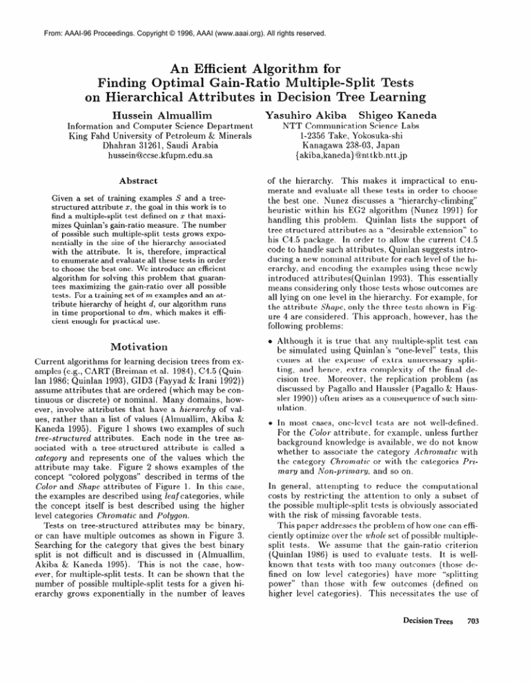
From: AAAI-96 Proceedings. Copyright © 1996, AAAI (www.aaai.org). All rights reserved.
Hussein
Almuallim
Information
and Computer Science Department
King Fahd University of Petroleum & Minerals
Dhahran 31261, Saudi Arabia
hussein@ccse.kfupm.edu.sa
Abstract
Given a set of training examples S and a treestructured attribute X, the goal in this work is to
find a multiple-split test defined on x that maximizes Quinlan’s gain-ratio measure. The number
of possible such multiple-split
tests grows exponentially in the size of the hierarchy associated
with the attribute.
It is, therefore, impractical
to enumerate and evaluate all these tests in order
to choose the best one. We introduce an efficient
algorithm for solving this problem that guarantees maximizing
the gain-ratio over all possible
tests. For a training set of m examples and an attribute hierarchy of height d,our algorithm runs
in time proportional
to dm, which makes it efficient enough for practical use.
Motivation
Current algorithms for learning decision trees from examples (e.g., CART (Breiman et al. 1984), C4.5 (Quinlan 1986; Quinlan 1993), GID3 (Fayyad & Irani 1992))
assume attributes that are ordered (which may be continuous or discrete) or nominal. Many domains, however, involve attributes
that have a hierarchy of values, rather than a list of values (Almuallim,
Akiba &
Kaneda 1995).
Figure 1 shows two examples of such
tree-structured attributes.
Each node in the tree associated with a tree-structured
attribute
is called a
cutegory and represents one of the values which the
attribute
may take. Figure 2 shows examples of the
concept “colored polygons” described in terms of the
Color and Shape attributes of Figure 1. In this case,
the examples are described using leafcategories,
while
the concept itself is best described using t)he higher
level categories
Chromatic and Polygon.
Tests on tree-structured
attributes
may be binary,
or can have multiple outcomes as shown in Figure 3.
Searching for the category that gives the best binary
split is not difficult and is discussed in (Almuallim,
Akiba & Kaneda 1995).
This is not, the case, however, for multiple-split
tests. It can be shown that the
number of possible multiple-split
tests for a given hierarchy grows exponentially
in the number of leaves
Uasuhiro
Akiba
Shigeo Kaneda
NTT
Communication
Science Labs
l-2356 Take, Yokosuka-shi
Kanagawa 238-03, Japan
{akiba,kaneda}@nttkb.ntt.jp
of the hierarchy.
This makes it impractical
to enumerate and evaluate all these tests in order to choose
the best one. Nunez discusses a “hierarchy-climbing”
heuristic within his EG2 algorithm
(Nunez 1991) for
handling t,his problem.
Quinlan lists the support of
tree-structured
attribut,es as a “desirable extension” to
his C4.5 package.
In order t#o allow the current C4.5
code to handle such attributes,
Quinlan suggests introducing a new nominal attribute for each level of the hierarchy, and encoding the examples using these newly
introduced att,ribut#es( Quinlan 1993). This essentially
means considering only t,hose tests whose outcomes are
all lying on one level in the hierarchy. For example, for
the attribute Shape, only the three tests shown in Figure 4 are considered.
This approach, however, has the
following problems:
Although it is true that any multiple-split
test can
be simulated using Quinlan’s
“one-level” tests, this
comes at) the expense of extra unnecessary
splitting, and hence, extra complexity
of the final decision tree.
Moreover, t(he replicat,ion problem (as
discussed by Pagallo and Haussler (Pagallo & Haussler 1990)) o ft en arises as a consequence of such simulation.
In most cases, one-level t,ests are not well-defined.
For the Color at#tribut#e, for example, unless further
background knowledge is available, we do not know
whether t,o associate the category Achromatic with
the category
Chromatic or with t,he categories Priand so on.
mary and Non-primary,
In general, at8temptting to reduce the computational
costs by rest8rict,ing t(he at,tention to only a subset of
the possible multiple-split, t)ests is obviously associat.ed
with the risk of missing favorable t,est,s.
This paper addresses the problem of how one can efficiently opt,imize over t#he whole set, of possible multiplesplit test,s.
We assume t(liat, t,lie gain-ratsi
criterion
(Quinlan 1986) is used to evaluate t,ests. It is wellknown t,hat tests with too many out,comes (those defined on low level cat.egories)
have more “split,ting
power” than t,hose with few outcomes
(defined on
higher level cat#egories).
This necessitates
the use of
Decision Trees
703
Any Shape
Non-convex
Convex
/\
Straight-lines
non-convex
Ellipse
Polygon
/I\
/\
Triangle Hexagon Square Proper
ellipse
/\
Circle
cross
star
Multiple-Split
Binary Test
Test
CUNY
non-convex
A
Kideny Crescent
shape
Figure
tribute
3: Binary
Shape
Figure
Shape
4:
and multiple
outcome
tests
on at-
Any Color
ChronZ/
\
Achromatic
Prim&/
Non-primary
\
A/
\\
Yellow Violet Orange
Figure
/I\
Black
Pink
White Gray
1: The Shape and Color hierarchies
( [ Yellow,
( [ Green,
( [ White,
( [ R-4
( [ Black,
Figure 2: Examples
Square
Hexagon
Cross
Circle
Circle
of the concept
a criterion such as the gain-ratio
penalty for excessive splitting.
] ,
] ,
] ,
+ >
+ )
- >
17
->
] ,
- )
“colored polygons”
that
involves some
We introduce an algorithm that, given a set of examples and a tree-structured
attribute x, finds a multiplesplit test defined on a: with maximized gain-ratio over
all possible multiple-split
tests defined on x. Our algorithm employs a computational
technique introduced
by Breiman et al. in the context of decision tree pruning (Breiman
et al. 1984).
The proposed algorithm
can be called from any top-down decision tree learning algorithm to handle tree-structured
attributes.
We
show that when the number of examples is m and the
depth of the hierarchy is d, our algorithm runs in time
proportional to dm in the worst case, which is efficient
enough from a practical point of view.
In the next section, we start by giving a precise
definition of the problem studied in this paper.
An
overview of the pruning algorithm of Breiman et al. is
then given, followed by an outline of our algorithm and
a discussion of its time complexity.
Finally, we conclude with a discussion of future research directions.
704
Learning
The
three
“one-level”
Problem
tests
for attribute
Definition
Let S be a set of training examples each having the
form [ (ul,uz,...,
a,), c 1, where al, ~2,. . . , a, are the
values of attributes
x1, x2, e. . , x,,
and c denotes a
class. Given such a set S, the basic operation in topdown induction of decision trees is to compute a score
for each xi, 1 5 i 5 n, that measures how good it is to
use xi for the test at the root of the decision tree being
learned for S. The attributes
~:i may be continuous,
discrete, and/or nominal. The objective of this work is
to extend this to tree-structured attributes such as the
Shape and Color attributes shown in Figure 1. A treestructured
attribute x E (~1, x2, . . . , z,} is associat,ed
with a hierarchy which we will denote by x-tree. Each
node in x-tree is called a category of 2. For simplicity, we assume that only the categories
at t.he leaves
of x-tree appear
in the examples
as values
of x. (See
Figure 2.)
Following (Haussler 1988), we define a cut, C, of Ptree as a subset! of the categories
of x satisfying
t,he
following two properties:
(i) For any leaf e of x-tree,
eit#her ! E C or e is a descendant
of some cat,egory
g E C. (ii) For any two categories ;,j E C, i is not,
a descendant) (nor an ancest$or) of j. Figure 5 shows
some cuts for the Shape hierarchy.
Each cut C of x-tree can be turned int,o a multiplesplit, test defined on x in a natural way. Namely, the
Any Shape
---I
-
Polygon --------Ellipse&
-
TI *iangle Hexagon Square
Figure
non-convex,
Proper
ellipse
Circle
=
-
2
Freyg7
‘)
X log,
(“7;’
“’ )
,
j=l
where Freq(j,S)
denotes the number of examples of
class j in S. The mutual information of a cut C for
at,tribut,e X, denoted MI(C), is defined as follows:
M(C)
= ‘);7
gEC
!Gfd
ISI
x Ent(Sg),
where S, is the subset of S having the outcome g of
for the attribut,e x. The split information
t,lie
for the cut, is defined as
cut,-c
Finally, the gain-ratio score foI the cut C with respect
t#oa training set S is given by
m?(C)
=
Ent(S) - MI(C)
With the above definitions,
statsed as follows:
SPF)
.
our problem
can
Star
I
non-convex
/\
Kideny -Crescent shape
cut
3
of cuts for the Shape hierarchy
5: Examples
outcome for each
test would have ICI outcomes-an
g E C, where an example in which z = v is of outcome
g iff v is a descendant of g, or ZJ is g itself. For example, Cut 3 in Figure 5 represents a test with the four
Icidney
outcomes { Con zle.r, Straight-lines-non-convex,
shape, Crescent}.
Clearly, the value of Shape in any example would belong to exactly one of these categories.
In this work, a test (cut) is evaluated using Quinlan’s
gain-ratio criterion.
For a given set S of examples with
q classes, let
Ent(S)
/\\
Cross
cut
now
be
Given a set of examples S and a tree-structured
at,tribut,e x with hierarchy x-tree, find a cut C of xtree such t,hat GR(C) is maximum over all possible
cuts of x-tree.
Not,e t,hat, cut,s consist,ing of “specific” categories (t#hose
t,liat, appear at, low levels of x-tree) give test#s with t,oo
many outcomes and consequently yield good MI scores
compared to cuts with more “general” categories which
naturally have fewer outcomes.
The use of gain-ratio
(rather than the pure gain or other similar measures)
helps in avoiding the t,endency towards those tests with
too many outcomes (Quinlan 1986).
It can be shown that the number of possible cuts for
a given hierarchy grows exponentially
in the number
of leaves of the hierarchy.
Thus, the challenge here is
t,o solve the above optimization
problem within affordable computational
costs. It turns out that this task
is very similar to the task of decision tree pruning. A
natural one-to-one correspondence
exists between cuts
and trees obtained by pruning x-tree. Namely, a cut C
is mapped to the pruned tree in which the subtrees
rooted at each g E C are removed (substituted
by
leaves).
Conversely, a pruned tree is mapped to the
cut C = {g I g is a leaf in the pruned tree}. This view
allows employing a decision tree pruning technique introduced by Breiman et al. (Breiman et al. 1984) in
solving our problem.
reirnan et alh
runing Algorithm
Breiman et al. present an efficient optimal pruning algorit,hm in which the goal is to minimize what they
call the cost-complexity
of a decision tree.
They assume that a decision t#ree T is given in which each test
node t is associated with an error est,imate e(t) which
measures the error int#roduced if the subtree below t is
substituted by a leaf. The error of a tree T’ obtained by
pruning subtrees from T is then defined as error
=
e
leaf
of
T,
e(e).
They
also
define
size(T’
)
as
the
numc
ber of leaves of T’. The quality of a pruned decision
t,ree T’ is measured as a linear combination
of its size
and error: Score, (T’) = error
+ Q siae(T’), for a
constant) Q > 0.
The goal in Breiman et al.‘s work is to find for each
o 2 0 a pruned t)ree that minimizes Score,.
Such a
tree is said to be optimally pruned with respect to Q.
Alt,hough o runs t#hrough a cont,inuum of values, only
a finit,e sequence of optimally pruned decision trees exDecision Trees
705
ists, where each tree minimizes Score, over a range of
01. Breiman et al. show that such a sequence can be
generated by repeatedly pruning at node t for which
the quantity
4
- I&L(t)
44
IL@)I - 1
is minimum, where L(t) denotes the set of leaves of the
subtree rooted at node t in the current tree. They call
this approach weakest link cutting.
Although Breiman et al. consider binary decision
trees only, extending their algorithm to decision trees
with multiple branches is straightforward
(Bohanec &
Bratko 1994). Moreover, in the setting of Breiman et
al., each leaf in a pruned tree contributes
a uniform
amount (exactly 1) to the size of the tree. Nevertheless, the same algorithm can be easily generalized by
associating a weight, w(t), with each node t in the given
tree T, and then letting size(T’) = Cl, leaf of T, w(e),
for a pruned tree T’. In this generalized setting, the
node t at which pruning occurs-is the node whickminimizes the quantity
44 - &L(t) 44
44 - w(t)*
c CEL(t)
Thus, generalized as above, the algorithm
et al. can be characterized
as follows:
of Breiman
8 Input: A decision tree T, with error estimate
and a weight w(t) at each node t in T.
* Output:
A sequence ((TGI),
(Et, 4,
(G,Q&
. a., (T,, a,.)}, such that each Ti is a pruned tree
that minimizes Score, in the range cri- 1 < cx < CY~,
where ~0 = 0, and CE,.= 00.
Although Breiman et al. only address the case of binary trees and uniform weight, their arguments
can
be extended to our generalized case of multiple branch
trees and non-uniform
weights.
Details are omitted
here, however, for lack of space.
Finding a Multiple-Split
Test with
Optimal Gain-Ratio
We now outline our algorithm for finding a test wit,h
maximum gain-ratio for a given set of examples S, and
a given attribute x with hierarchy x-tree. The first step
of the algorithm is an initialization
step:
Step I: For each category g in x-tree, attach an
array CD, to be used to store the class distribution
at that category. This array has an entry for each
class which is initially set to 0. We repeat the
following steps for each example e E S:
1. Let 21be the value of at,tribute
x in e.
2. Let cl be the class of e.
3. Increment
CD, [cl].
4. Climbing from v towards
CD,[cl] for every ancestor
706
Learning
At the end of Step I, each array CD, will be storing the
class distribution
for those examples in S in which the
value of the attribute x is a descendant of the category
g. The next step computes the amounts each category
g would contribute
to MI(C)
and Sp(C) if g were a
member in a cut C.
For each category g in x-tree, let IS,I =
is, the number of examples in
which the value of attribute
x is a descendant of
g), and compute the following two quantities:
Step
II:
cc C4kl P a t
i(g)
-zF
y
X log:,
(v)
9
s(g) = #
x
9
log,,
(E)
Now for any cut C, it is obvious that MI(C)
and
Sp(C) (as defined in Section 2) can be computed as
s(g), respectively.
The next step
is a call to the generalized algorithm of Breiman et al.:
C;ECiis) andEYCYC
Step III: Pass the tree x-tree to the generalized
Breiman et al.‘s algorithm, viewing each i(g) and
s(g) as the error estimate and the weight of node
g , respectively.
As explained previously, there is a one-to-one
correspondence between the set of all possible cuts and the
set of all possible pruned decision trees. Since we are
passing i(g) and s(g) to Breiman et al.‘s algorithm
as the error estimates
and the weights at the nodes,
error
and size( T’ ) are respectively
equivalent
to
MI(C) and Sp(C), for the cut C corresponding
to T’.
This then justifies the following view:
Step IV: View the tree sequence returned by
Breiman et al.‘s algorithm as a sequence ((Cl, al),
(C2, cq), ((2’3, CQ), . . . , (C,, a,.)}, in which each Ci
minimizes Score, (C) = 1MZ(C) + 0 Sp(C) over all
cuts
where
C , within the range
a() = 0 and cy, = 00.
The cut sequence we now have at hand is not directly
maximizing the gain-ratio, but rather optimizing under
a different criterion (hill(C) + Q Sp(C)) which involves
the unspecified parameter
CY. However, the following
theorem puts things in perspective:
Theorem:
In the sequence {Cl, C’, . . . , C,.-1) of cuts
produced by employing the algorithm of Breiman et al.,
there exists a cut with maximum gain-ratio.
Proof: This is shown by contradiction.
Suppose none
of the produced cuts maximizes the gain-ratio.
Then,
there exists some cut C* such that, for all 1 5 i 5 T- 1,
we have GR(C*)
> GR(Ci),
that is
Ent(S)
the root, increment
g of 21 in x-tree.
=
- MI(C*)
Su(C*)
> Ent(S) - M1(ci),
SP(Ci)
1< i < r _ 1
*
(1)
Consider
now the following
ct
value of o:
= Q1 = JWS)
- Mw*)
Sp(C*)
-
For any cut C, it is true that E&(S) > MI(C). Therefore, al is a legitimate value for a since it is greater
than or equal to 0. At this particular value for o,
Score, 1(C”)
=
MI(c*)
=
Ent(S).
+ @qjg!pJ
x sP(c*)
-’ ’
On the other hand, for any i, 1 5 i 5 r - 1,
Score,,(G) =
MI(Ci) + v
>
WG)
=
Ent(S).
x sp(ci)
+ ,=$&$Q
- .
id
x Sp(C,)
(from(1))
The above means that at oi we have Score,, (C” ) <
Score,, (Ci) for all Ci in {Cl, C2, C’s, +. aC.-i}.
This is
a contradiction
since for any value of cy > 0, one of the
cuts in { Ci, Cz, C3, . . . C,- 1) must minimize Score,, .O
The above theorem
leads to the following final step.
Step V: Compute the gain-ratio for each Ci, 1 5
i 5 r - 1 and return the cut with maximum gainratio among these.’
Various details have been omitted in the above outline of our algorithm in order to simplify the discussion.
In an actual implementation,
Steps III and IV (finding the sequence of cuts) and Step V (computing the
gain-ratio scores) can be run concurrently-each
time
a cut is generated,
its gain-ratio is computed, and the
cut is kept if its gain-ratio is the highest so far. In the
appendix, we give a full pseudo-code description of the
algorithm in which the weakest-link cutting algorithm
of Breiman et al. is embedded.
Time
Complexity
Analysis
Let m be the number of examples and q the number
of classes. Let the number of leaves of x-tree be s and
let its height be d. Assume that each node in x-tree
has at m&t k children.
Then, it can be shown that
the implementation
given in the appendix runs in time
O(dm + (q + kd)s).
We can, however, assume that
s 5 m, since if this is not the case, then this means
that some of the leaf categories in x-tree never show up
in any example in S. In such a case, one can reduce
the hierarchy by just ignoring these. More precisely, a
category in x-tree is considered if and only if it is an
ancestor of some leaf category that appears in at least
one example in S. Reducing x-tree in this manner results in a hierarchy of at most m leaves. Thus, the time
‘Note that the test corresponding
ing since it has only a single outcome
to C, is not interestand does no splitting.
complexity of our algorithm is in fact O((q + kd)m) in
the worst case.
It is interesting
to note that the above bound is
only linear in the height of the hierarchy.
Therefore,
when dealing with somewhat balanced hierarchies,
d
becomes
in the order of logs, which is in turn in
the order of log m. This then gives time complexity
S ince the number of classes,
of O((q+
klogm)m).
q is usually small compared to klog m, this can be
viewed as 0 (km log m). Interestingly
enough, this is
similar to the time complexity of 0( m log m) for the
task of handling continuous attributes
(Quinlan 1986;
Fayyad & Irani 1992).
Conclusion
and
For a given tree-structured
attribute,
the goal of this
work is to find a multiple-split
test that maximizes
Quinlan’s gain-ratio
measure with respect to a given
set of training examples.
We presented an algorithm
that achieves this goal and runs in time linear in the
number of training examples times the depth of the
hierarchy associated with the tree-structured
attribute.
In no way one can claim any superiority of multiplesplit tests in generalization
performance
over other
kinds of tests, such as binary tests that are based
on a single value of the attribute
(See Figure 3). In
fact, multiple-split
tests and binary tests should not
be viewed as mutually exclusive choices. One indeed
can find the best multiple-split
test using our method,
and in parallel, find the best binary split test using the
method of (Almuallim,
Akiba & Kaneda 1995), and
finally choose from these the test with higher score.
The gain-ratio criterion of Quinlan is “hard-wired”
in our algorithm.
It would be interesting to generalize
the algorithm to cover other similar measures as well.
It is also interesting
to consider tests that group different values of a tree-structured
attribute in a single
outcome. This kind of tests is studied in (Fayyad 1994;
Fayyad & Irani 1993; Quinlan 1993) for other attribute
types. Finally, in certain applications,
attributes
may
be associated
with directed acyclic graphs (DAG’s)
rather than trees as assumed in our work. Studying
this generalized
problem is an important
future research direction.
Acknowledgment
Hussein Almuallim
thanks King Fahd University
of
Petroleum & Minerals for their support. This work was
partially conducted during his visit to Prof. Shimura
Lab. of Tokyo Institute of Technology,
sponsored by
Japan’s
Petroleum
Energy Center.
Thanks
also to
Hideki Tanaka of NHK, Japan for a useful discussion.
Appendix
Our algorithm is described below in pseudo code. All
the variables are assumed global. i[g] and s[g] are computed for each node g in line 2.1 of FindBestCut.
At
each node g, o[g] stores the value of (Y above which
Decision Trees
707
the subtree rooted at g is pruned. This is initialized
at lines 2.2.4 and 2.3.4 of FindBestCut.
Each call to
PruneOnce results in pruning the subtree rooted at g
for which ab] is minimum over all (unpruned)
nodes
of T. At that time, the flag Pruned[g] becomes True
and cy[s] is updated for all ancestors s of g.
The variable SmaZZest.a.BeZow[g] stores the smallest Q value over all descendant
of g. This variable
is stored in order to efficiently locate the node with
minimum o in the current tree in each pruning iteration.
SubTreeMl[g] and SubTnzeSp[g] store the sum
of i[e] and s[!!], respectively, for all leaves l of the current subtree rooted at g. These are initialized in step 2
of FindBestCut,
and then updated in step 10 of PruneOnce each time pruning occurs at a descendant
of
g. The current best cut is kept track of by the flag
InBestCut[g].
A node g is in the current best cut if
this flag is True for g and False for all its ancestors.
Algorithm
FindBestCut
Input: A sample S, an attribute x, its hierarchy T
1.
Initialize the arrays CD as in STEP I.
2.
Traverse T in post-order.
For each g in T:
2.1.
Compute i[s] and s[s] as in STEP II.
2.2.
If g is a leaf then
Pruned[g] = True
2.2.1.
2.2.2.
Sub TreeMflg] = i[s]
2.2.3.
SubTreeSp[g] =s[g]
2.2.4.
491 =CX3
Smallesta. BeZow[g] = 00
2.2.5.
InBestCut[g] = True
2.2.6.
else
2.3.
Pruned[g] = False
2.3.1.
2.3.2.
SubTreeMl[g] = Cy:=hild of 9 SubTreeMl[y]
2.3.3.
SubTreeS&]
= Cy:child
ofg SubT~eSz&d
2.3.4.
[
491 = k;-+;::$geF-$;]
2.3.5.
SmaZZest.cr.BeZow 1g] = min {a[g],
min{ SmaZZest.a.BeZow[y] jy is a child of g}}
InBestCut[g] = False
2.3.6.
4.
5.
5.1.
p = PruneOnce
While p # root of T:
ThisGR=
i[root
--
-
-
of T]-SubTreeMqroot
SubTreeSp[root
of T1
of T]
If ThisGR 2 BestGR then
5.2.
BestGR = ThisGR
5.2.1.
InBestCutb]
= True
5.2.2.
p = PruneOnce
5.2.3.
Report BestGR as the best gain-ratio over all
6.
cuts of T
Report the set {g 1 InBestCut[g] = True and for
7.
every ancestor g’ of g, InBestCut[g’] =FuZse} as
the best cut.
Procedure PruneOnce
1.
Let g = root of T
2.
While a[g] > SmuZZest.cr.BeZow[g] :
2.1.
g’ = child of g such that
708
Learning
SnluZZest.a. BeZow[g’] is minimum
I
2.2.
3.
Pru$;{]
4.
5.
6.
7.
8.
9.
10.
10.1.
10.2.
491
= True
co
Sm ZZest.cr.BeZow[g] = 00
Su f-TreeMl[g] = i[g]
Sub TreeSp[s] = s[g]
p=g
root of T, return p
Ifp=
Repeat
g = parent of g
>ub?reeMl[g]
i Cy:child of 9 SubTreeMfly]
10.3.
SubTr=%[gl
10.4.
@[sl= ~~-$~eJ$~!~~~
= &.child
of g SubTreeSlobl
SmuZZest.a.BeZow 1g] = min{ob],
min{ SmuZZest.ar.BeZow[g’] ] g’ is a kid of g}}
10.6. until g = the root of T
11.
Return p
10.5.
References
Almuallim, H.; Akiba, Y.; and Kaneda, S. 1995. On
Handling Tree-Structured
Attributes in Decision Tree
Learning. In Proceedings
of the 12th International
Conference on Machine Learning, p. 12-20. San Francisco, California:
Morgan Kaufmann.
Bohanec, M.; and Bratko,
for Simplicity in Decision
15~223-250.
I. 1994. Trading
Trees. Machine
Accuracy
Leurning,
Breiman,
L.; Friedman,
J.H.;
Olshen,
R.A.;
and
Stone, C.J. 1984. Classification and Regression Trees.
Belmont:
Wadsworth.
Fayyad, U. M.; and Irani, K. B. 1992. On the Handling of Continuous
Valued Attributes
in Decision
Tree Generation.
Machine Learning, 8:87-102.
Fayyad, U. M.; and Irani, K. B. 1993. Multi-Interval
Discretization
of Continuous-Valued
Attributes
for
Classification
Learning. In Proceedings of the 13th International Joint Conference on Artificial Intelligence,
p. 1022-1027.
Fayyad, U. M. 1994. Branching
on Attribute
Values
in Decision Tree Generation.
In Proceedings
of the
12th National Conference
on Artificial Intelligence,
p. 601-606.
Haussler, D. 1988. Quantifying
Inductive
Bias:
AI
Learning Algorithms
and Valiant’s Learning Framework. A rtificiul Intelligence, 36: 177-22 1.
Nunez, M. 1991. The Use of Background
KnowlMachine Learning,
edge in Decision Tree Induction.
6: 231-250.
Pagallo, G.; and Haussler, D. 1990. Boolean Feature
Discovery in Empirical
Learning. Machine Learning,
5( 1):71-100.
Quinlan, J. R. 1986. Induction
chine Learning, 1( 1):81-106.
Quinlan, J. R. 1993. C4.5:
Learning, p. 104. San Mateo,
of Decision
Trees. Mu-
Programs for Machine
CA: Morgan Kaufmann.