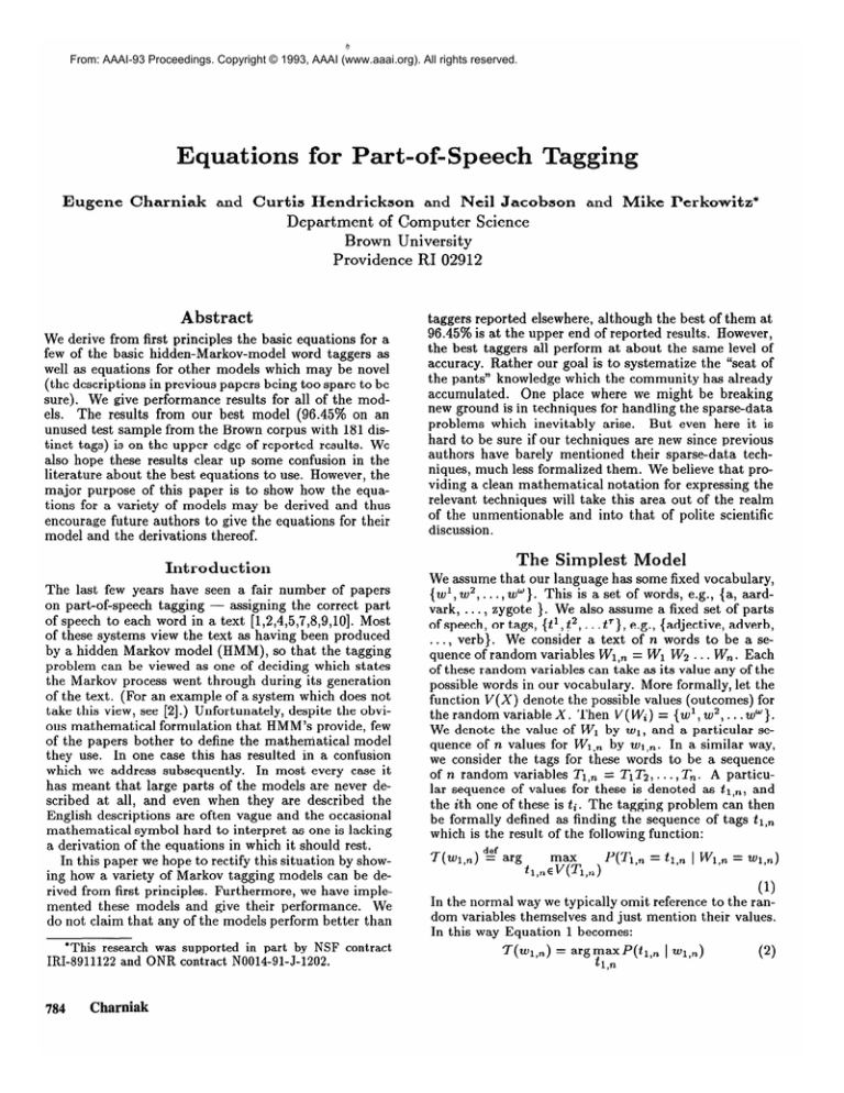
From: AAAI-93 Proceedings. Copyright © 1993, AAAI (www.aaai.org). All rights reserved.
Equations
Eugene
Charniak
for Part-of-Speech
and Curtis Hendrickson
and Neil Jacobson
Department of Computer Science
Brown University
Providence RI 02912
Abstract
We derive from first principles the basic equations for a
few of the basic hidden-Markov-model word taggers as
well as equations for other models which may be novel
(the descriptions in previous papers being too spare to be
sure). We give performance results for all of the models. The results from our best model (96.45% on an
unused test sample from the Brown corpus with 181 distinct tags) is on the upper edge of reported results. We
also hope these results clear up some confusion in the
literature about the best equations to use. However, the
major purpose of this paper is to show how the equations for a variety of models may be derived and thus
encourage future authors to give the equations for their
model and the derivations thereof.
The last few years have seen a fair number of papers
on part-of-speech tagging - assigning the correct part
of speech to each word in a text [1,2,4,5,7,8,9,10]. Most
of these systems view the text as having been produced
by a hidden Markov model (HMM), so that the tagging
problem can be viewed as one of deciding which states
the Markov process went through during its generation
of the text. (For an example of a system which does not
take this view, see [2].) Unfortunately, despite the obvious mathematical formulation that HMM’s provide, few
of the papers bother to define the mathematical model
they use. In one case this has resulted in a confusion
which we address subsequently. In most every case it
has meant that large parts of the models are never described at all, and even when they are described the
English descriptions are often vague and the occasional
mathematical symbol hard to interpret as one is lacking
a derivation of the equations in which it should rest.
In this paper we hope to rectify this situation by showing how a variety of Markov tagging models can be derived from first principles. Furthermore, we have implemented these models and give their performance. We
do not claim that any of the models perform better than
*This research
was supported
in part by NSF
IRI-8911122
and ONR contract
NO01491-J-1202.
Charniak
and Mike Perkowitz*
taggers reported elsewhere, although the best of them at
96.45% is at the upper end of reported results. However,
the best taggers all perform at about the same level of
accuracy. Rather our goal is to systematize the “seat of
the pants” knowledge which the community has already
accumulated. One place where we might be breaking
new ground is in techniques for handling the sparse-data
problems which inevitably arise. But even here it is
hard to be sure if our techniques are new since previous
authors have barely mentioned their sparse-data techniques, much less formalized them. We believe that providing a clean mathematical notation for expressing the
relevant techniques will take this area out of the realm
of the unmentionable and into that of polite scientific
discussion.
The Simplest
Introduction
784
Tagging
contract
Model
We assume that our language has some fixed vocabulary,
{ wl, w2,. . . , ww}. This is a set of words, e.g., {a, aardvark, . . . . zygote ). We also assume a fixed set of parts
of speech, or tags, {t’, t2, . . .t’}, e.g., {adjective, adverb,
..‘, verb}. We consider a text of n words to be a sequence of random variables VVI,~= Wi lV2 . . . IV,. Each
of these random variables can take as its value any of the
possible words in our vocabulary. More formally, let the
function V(X) denote the possible values (outcomes) for
the random variable X. Then V(Wi) = {w’, w2,. . . ww}.
We denote the value of Wi by 201, and a particular sequence of n values for l~Vi,~ by ~1,~. In a similar way,
we consider the tags for these words to be a sequence
of n random variables 7’1,~ = TiT2, . . . , Tn. A particular sequence of values for these is denoted as t~,~, and
the ith one of these is ti . The tagging problem can then
be formally defined as finding the sequence of tags ti ,ra
which is the result of the following function:
I(w~,~) def arg
max
h,,d(Tl,n)
JV’l,n
= h,n I W,n = WI+)
(1)
In the normal way we typically omit reference to the random variables themselves and just mention their values.
In this way Equation 1 becomes:
7(wl,n)
= argylyP(tl,n
,
I ~1,~)
(2)
We now turn Equation 2 into a more convenient form.
T(qn)
=
argf211;
P(h,n,
(3)
p(wl,n)
,
=
w,n)
wy-y;P(tl,n,
,
~(Wl,n)
Wl,ta).
9 W,n)
=
I w)P(w2
I t1,
P(tn
w,2)
I h,
P(Wl)P(h
n
w)
Wl,?a-1)
I t l,n,
(5)
W,n-1)
I w)
qwi It
1$-l,
w,i--1)
i=2
P(ts
1 tl,i-1,
w,i)
(6)
n
=
P(‘wi
I h,i-1,
w,i-1)
i=l
qti I h,i-1,
Wl,i)
(7)
Here we simplified Equation 6 to get Equation 7 by suitably defining terms like tl,o and their probabilities. We
derived Equation 7 by first breaking out P(wl) from
In a similar way we can first break out
P(tl,n,
Win).
P(tl), giving this:
n
P(tl,n,
W,7a)
qti
=
1 b,i-1,
w,i-1)
a=1
P(wi
I tl,i,
qi-1)
(8)
All of our models start from Equations 7 or 8, or, when
we discuss equations which smooth using word morphology, modest variations of them.
Up to this point we have made no assumptions about
the probabilities we are dealing with, and thus the probabilities required by Equations 7 and 8 are not empirically collectible. The models we develop in this paper
differ in just the assumptions they make to allow for the
collection of relevant data. We call these assumptions
“Markov assumptions” because they make it possible to
view the tagging as a Markov process. We start with
the simplest of these models (i.e., the one based upon
the strongest Markov assumptions).
We start with Equation 7 and make the following
Markov assumptions:
qwi
I h,i-1,
P(h I t l,i-1,
w,i-1)
Wl,a 3
;a$
P(w
’
I w,i-1)
i=l
=
P(w
=
P(t,
I w,i-1)
1 Wa)
(9)
(10)
I Wi)
(11)
n
p&i I w)
(12)
Equation 12 has a very simple interpretation. For each
word we pick the tag which is most common for that
word. This is our simplest model.
Estimation
***
I h,n-1,
qwn
=
arg
P(fi
P(w)P(h
qt2
=
(4
In going from Equation 3 to 4 we dropped P(w~,~) as it
is constant for all ti,, .
Next we want to break Equation 4 into “bite-size”
pieces about which we can collect statistics. To a first
approximation there are two ways this can be done. The
first is like this:
P(fl,n
Substituting these equations into Equation 7, and substituting that into Equation 4 we get:
of
Before one can use such a model however, one still needs
to estimate the relevant parameters. For Equation 12
we need the probabilities of each possible tag for each
possible word: P(t” ] &). The most obvious way to get
these is from a corpus which has been tagged by hand.
Fortunately there is such a corpus, the Brown Corpus [6]
and all of the statistical data we collect are from a subset
of this corpus consisting of 90% of the sentences chosen
at random. (The other 10% we reserve for testing our
models.) So, let C(t”, wj) be the number of times the
word w3 appears in our training corpus with the tag t”.
In the obvious way C(wj) = Cd C(t”, 203). Then one
approximation to the statistics needed for Equation 12
is the following estimate:
est C(ti)
P(t” I UFi) =
C(wj)
W’)
*
However, Equation 13 has problems when the training
data is not complete. For example, suppose there is no
occurrence of word w u?. First, the quotient in Equation
13 is undefined. As this is a problem throughout this
paper we henceforth define zero divided by zero to be
zero. But this still means that P(t” I w”) is zero for all
t”.
We solve this problem by adding further terms to
Equation 13. We model this after what is typically done
in smoothing tri-gram models for English [7]. Thus we
add a second term to the equation with weights attached
to each term saying how heavily that term should be
counted. That is, we are looking for an equation of the
following form:
.
.
P(V I WJ) “At AI
c&yy
+ X2(wj)f(t”,
w-q.
(14)
Here f(ti, d) is standing in for our as yet to be disclosed
improvement. The two Xs are the weights to be given to
each term. Note that they can be different for different
w and thus we have made them functions of &. For any
w Equation 14 must sum to one over all t”. We ensure
this by requiring that the As sum to one and that the
terms they combine do so as well.
Statistically-Based
NLP
785
If we are primarily concerned about estimating
P(ti 1wj ) for & which have not been encountered before
the is can take a particularly simple form:
1
0
if C(wj) 2 1
otherwise.
(15)
With these Xs the second term of Equation 14 should
be the probability that a token of a word & which we
have never seen before has the tag t’. Obviously we cannot really collect statistics on something that has never
occurred: however when we were gathering our count
data in the first place we often encountered words which
up to that point had not been seen. We collect statistics
on these situations to stand in for those which occur in
the test data. Thus, let C,(t”) be the number of times a
word which has never been seen with the tag- t” get
this
tag, and let Cn() be the number of such occurrences in
total. Then our improved probability estimation equation is this:
P(ti
I wj) zt X&d)
C(@, wj)
+
c(wj)
xz(-j)~
n
(16)
With this improved parameter estimation function we
are now able to collect statistics from our corpus and test
the model thereby derived on our test corpus. The results are quite impressive for so simple a model: 90.25%
of the words in the test data are labeled correctly. (The
data for all of the models is summarized at the end of
the paper in Figure 2.)
The “Standard”
I h,i-lP-qi--1)
P(Wi
I t l,i,
w,a-1
>
=
P(k
=
P(w
I h-1)
I h,i)
(17)
(18)
That is, we assume that the current tag is independent
of the previous words and only dependent on the previous tai. Similarly we assume that the correct word is
independent of everything except knowledge of its tag.
With these assumptions we get the following equation:
T(Wl,n)
=
argmaxfi
‘l,n
P(t; I ta-l)P(wi
I ti)
(19)
j=l
This equation, or something like it, is at the basis of
most of the tagging programs created over the last few
years. One modification expands P(ti I ti-1) to take into
consideration the last two tags [4,7]. Experimentation
has shown that it offers a slight improvement, but not a
great deal. We ignore it henceforth. Another modification conditions the tag probability on the tags following
the word rather than those which preceded it [4]. However, it is easy to show that this has no effect on results.
786
Charniak
T(Wl,n)
=
argr;fi
P(ti
I td-l)P(td
I w;).
(20)
, j= 1
The difference is in the last term. This equation is found
in [4,9] and is described in words in [5]. (However, while
Church gives Equation 20 in [4], the results cited there
were based upon Equation 19 (Church, personal communication) .)
Equation 20 seems plausible except that it is virtually
impossible to derive it from basic considerations (at least
we-have been unable to do so). Nevertheless, given the
drastic Markov assumptions we made in the’derivation
of Equation 19 it is hard to be sure that its comparative
theoretical purity translates into better performance. Indeed, the one paper we are acquainted with in which the
comparison was made [l] found that the less pure Equation 20 gave the better performance. However, this was
on a very small amount of training data, and thus the
results may not be accurate.
To determine which, in fact, does work better we
trained both on 90% of the Brown Corpus and tested
on the remainder. We smoothed the probabilities using
Equation 16. To use this on Equation 19 we made the
following change in its form:
n
I(Wl,n)
=
argmax
P(G
Model
The model of Equations 12 and 16 does not take any
context into account. It simply chooses the most likely
tag for each word out of context. Next we develop a
model which does take context into account.
This time we start from Equation 8 and simplify it by
making the following two Markov assumptions:
qti
A more important difference is that many do not use
Equation 19 or the just-mentioned variants, but rather:
I h-1)
P(w,)pqlt; I 4
=
arg;-fi
P(ta I t~-~)‘$,i
,
d=l
(21)
7)
i
(22)
It was also necessary to smooth P(ta 1ti-1).
In particular we found in our test data consecutive words with
unambiguous tags, where the tags had not been seen consecutively in the training data.‘-To overcome this problem in the simplest fashion we smoothed the probability
as follows:
P(ta I t&l)
e
(1 - c)C$-“:’
d- 1
+ c.
(23)
Here E is a very small number so that its contribution
is swamped by the count data unless that contributes
zero. The net effect is that when there is no data on tag
context the decision is made on the basis of P(d
I ti) in
Equation 19 or P(t’ I wj) in Equation 20.
The results were unequivocal. For Equation 19 we got
95.15% correct while for the less pure Equation 20 the
results were poorer, 94.09%. While this may not seem
like a huge difference, a better way to think of it is that
we got an 18% reduction in errors. Furthermore, given
that the models have exactly the same complexity, there
is no cost for this improvement.
An Improved
Smoothing
Model
The smoothing model of Eq uation 16 is very crude. This
and the subsequent section improve upon it. One problem is that the model uses raw counts to estimate the
probabilities for a word’s tags once it has seen a word,
even if only once. Obviously, if we have seen a word, say,
100 times, the counts probably give a good estimate, but
for words we have seen only once they can be quite inaccurate. The improvement in this section is concerned
with this problem.
In Equation 16 we collected statistics on the first occurrences of words we saw in the training data and used
these statistics to predict what would happen on the first
occurrences of words we saw in the test data. To improve our model we try to estimate the probability that
we will next see the tag t” as the tag for & despite the
fact that it has never appeared as the tag for d before
- P(t”-new I wj).
P(t”-new
I wj) “At
{
if C(t”, wj) > 1 0
otherwise
P(new tag ] C(wj))P(t”
I new tag)
(24)
The first line states that that t” cannot be new if it has
already appeared as a tag of wj. The second line says
that we approximate the probability by assuming independence of the “newness” and the fact that it is the ith
tag. Second it assumes that the probability of newness
is only dependent on how many times we have seen wj
before. Also, rather than collect P(new tag I C(wj)) for
all possible C(wJ), we have put counts into the following
equivalence categories based upon how many times the
word has been seen: 0, 1, 2, 3-4, 5-7, 8-10, 11-20, 21-36,
30-up. Let N(C(wj))
denote the frequence class for wJ.
Then
P(new tag I C(wj))
“AtP(new tag I N(C(wj)))
(25)
We can now use P(t”-new ] wj) to smooth P(t” I wj) in
Equation 16, giving us:
. .
p(ti 1wj) ?2 xl(wj) c:i;y;J
P(t”-new
I wj)
However, Xi and A2 cannot retain their definitions
from Equation 15 as that assumed that any word we
had seen would use the direct counts rather than the
Cn’s. One way to get the new Xs is to use extra training
data to train the HMM corresponding to Equations 22
and 26 to find a (locally) best set of X-values as done
in [7]. However, it is possible to provide an argument
for what their values ought to be. If we think about an
HMM for producing the part of speech given the word,
for each word there would be arcs leaving the state corresponding to each possible tag. (In fact, there would be
several arcs for each tag, each going to a different next
state, but we ignore this.) This would appear as shown
Figure 1: A Markov model for P(t” I wj)
on the upper portion of Figure 1. We assume that for
wj we have seen v of the tags, t1 to t”, and the rest,
t”+l to tT, have not been observed for wj. The idea of
Equation 26 is that the first term estimates the probabilities associated with the arcs t1 to t”, and the second
term estimates the rest. To make the HMM look more
like this equation we can transform it into the form on
the lower portion of Figure 1 where we have introduced
two E (no.output) transitions with probabilities Xi(wj)
and &(wJ), respectively. From this HMM it is easier to
see the significance of these two probabilities: Xr(wj) is
the probability that the next occurrence of WJ has as an
associated tag, a tag which has occurred with wj before,
and Xz(wj) is the probability that it is a new tag for wJ.
This latter term is the sum in the denominator of the
second term of Equation 26.
Morphological
The second improvement to our smoothing function uses
the word-ending information to help determine correct
tags. For example, if we have never seen the word “rakishly,” then knowledge that “1~” typically ends an adverb
will improve our accuracy on this word - similarly, for
“randomizing.”
We do not want to tackle the problem of determining
the morphology of English words in this paper. Rather
we assume that we have available a program which assigns roots and suffixes (we do not deal wit h any other
kind of morphological feature) to our corpus and does so
Statistically-Based
NLP
787
as well for those words in our test corpus which have appeared in the training corpus. For the words in the test
corpus which have not appeared in the training corpus
the morphological analyzer produces all possible analyses for that word and part of the problem we face is
deciding between them. We should note that the morphological analyzer we had was quite crude and prone
to mistakes. A better one would no doubt improve our
results.
To accommodate our morphological analysis we now
consider probabilities for different- root-suffix combinations. Following our earlier conventions, we have a set
of roots {rl, . . . . rp) and a set of suffixes {sl, . . . , so).
f1.n and s1.n are sequences of n roots and suffixes with
ri’and sa being the ith one of each.
=
I(Wl,n)
argmax
tl n
t
C
I W,n)
P(tl,n~~l,n~Sl,n
rl,n,Sl,n
(27)
=
P(h
arg max
tl,n
,nt fi,n,
>:
Sl,n,
W,n
>
p(wl,n)
rl,nA,n
(28)
=
arg max
tl n
9
>:
rl,n,
P(tl,n,
Sl,n,
W,n)
ri,n,Si,n
(29)
=
=
arg max
tl n
):
7 rl,nA,n
arg max
P(tl,n,
rl,n9Sl,n)
(30)
zl,n
C
fi P(ti 1tl,i--1, rl,i-1, qi-1)
rl,n,Sl,n i=l
P(ri, si 1tl,i, rl,i-1, qi-I)
(31)
We delete wr ,n in going from Equation 28 to 29 because
roots nlus suffixes determine the words. However, this
means that in all of the equations after that point there
is an implicit assumption that we are only considering
root as suffixes which combine to form the desired word.
Next we make some Markov assumptions.
L
With these assumptions we can manipulate Equation
31 as follows:
n
7(w1,~)
=
argmax
t19n
P(ri,
I t 1+-l,
qi-1,
qi--l
Si 1 tl,i,
rl,i-1,
Sl,i-1)
P(ri,
Sj
P(ti
I=
I t;)
1 b-1)
=
P(ri,
Si I ti)
=
P(ri
1 ti)P(&
(32)
(33)
I ti)
(34
The first two are just the ones we made earlier, but now
with the roots and suffixes broken out. Equation 34 is
new. It can be interpreted as saying that knowing the
root does not help determining the suffix if we know the
part-of-speech of the word. This is probably a reasonable
assumption, particularly compared to the others we have
made.
788
Charniak
n
Pl,n,Sl,n
i=l
P(ti
I ii-l)
P(SiI ti)P(ri l ii)
(35)
n
=
arg max
tl n
’
c
rl,ntSl,n
j-J ws I ti-l)P(Si
I ti)
i=l
Equation 36 is a version of Equation 19, but adapted
to morphological analysis. It differs from the earlier
equation in three ways. First, it includes a new term,
P(si I ti), for which we now need to gather statistics.
However, since the number of tags and suffixes are small,
this should not provide any difficult sparse-data problems. Second, rather than needing to smooth P(t” I wj)
as in Equation 19, we now need to smooth P(t” I d).
However, it seems reasonable to continue to use Equation 26, with rj substituted for &. Finally, there is the
term P(ri), and this deserves some discussion.
There was no term corresponding to P(ri) in Equation
as the term which would have correspbn’ded to it was
wi), and that was removed as it was the same for all
ta&. However, in Equation 36 we are summing over
roots, so P(ri) is not a constant. In particular assuming
that we would want our program to interpret some new
word, e.g., “rakishly” as “rakish” + “ly,” (or even better,
“rake” + “ish” + “ly,” if our morphological analyzer
could handle it) it would be the P(.ri) term which would
encourage such ‘a preference in Equation 36. It would do
so because the probability of the shorter root would be
much higher than the longer ones.
To model P(ri) we have adopted a spelling model
along the lines of the one used for the spelling of unknown words in [3]. Th is combines a Poisson distribution over word lengths with a maximum at 5, times a
distribution over letters. We adopted a unigram model
for letters. Here I rj I is the length of rj and Zi is the ith
letter of 7-j.
P(d)
P(h
C
5’r3’ -5 ‘2
Et ne
I’
I’
p(li
I &,l)
(37)
k=l
Results
The results of our experiments are summarized in Figure 2. We trained our models on the Brown corpus
with every tenth sentence removed (starting with sentence 1) and tested on these removed sentences. There
were 114203 words in the test corpus. For the more basic methods we did experiments on both the full Brown
corpus tag set (471 different tags) and a reduced set (186
tags). (Most of the tags in the full set are are “complex”
tags’in‘that they consist of a basic tag plus one or more
Equations
12 and 16
20, 16, and 23
19, 16, and 23
19, 26, and 23
36, 26, and 23
% Correct
471 Tags
90.25
94.09
95.15
% Correct
186 Tags
91.51
95.04
95.97
96.02
96.45
Figure 2: Results obtained from the various models
tag modifiers. For those familiar with the Brown Corpus, to get the reduced set we stripped off the modifiers
“F W” (foreign word), “TL” (title), “NC” (cited word),
and “HL” (headline). For the more complex techniques
we only used the reduced set since the basic dynamic
programming algorithm for finding the best tags runs in
big-0 time = r2 where r is the number of different tags.
Using normal tests for statistical significance we find that
for the interesting cases of Figure 2 a difference of .l%
is significant at the 95% level of confidence.
Certain results are clear. One can get 90% of the tags
correct by just picking the most likely tag for each word.
Improving the model to include bigrams of tags increases
the accuracy to the 95% level, with the more theoretically pure P(wi ] ti) performing better than P(ti ] wi),
contrary to the results in [l]. Furthermore the improvement is much larger than the .l% required for the 95%
significance level. Improvement beyond this level is possible but it gets much harder. In particular, the improvement from the more sophisticated smoothing equation,
Equation 26 is minimal, only .05%. This is not statistically significant. However, there is reason to believe
that this understates the usefulness, of this equation. In
particular we believe that the very crude 23 is causing extra errors when combined with the improved smoothing.
Equation 23 combined with the crudeness of our morphology component also limited the improvement shown
in the last line of Figure 2. Also, we should really treat
endings as tag “transformers,” something Equation 36
does not do. The combination of these three debilitating factors caused frequent errors in known words,
and thus the figure of 96.45% was obtained when we
treated known words as morphologically primitive. This
improvement is statistically significant. We believe that
fixing these problems would add another tenth of a percent or two, but better performance beyond this will
require more lexical information, as that used in [lo].
However, the point of this paper was to clarify the
basic equations behind tagging models, rather than improving the models themselves. We hope this paper encourages tag modelers to think about the mathematics
which underly their models and to present their models
in terms of the equations.
References
1. BOGGESS, L., AGARWAL, R. AND DAVIS, R. Disambiguation of prepositional phrases in automatically
labelled technical text. In Proceedings of the Ninth
National Conference on Artificial Intelligence. 1991,
155-159.
2. BRILL, E. A simple rule-based part of speech tagger.
In Proceedings of the Third Conference on Applied
Natural Language Processing. 1992.
3. BROWN,
P. F., DELLA PIETRA, S. A., DELLA
PIETRA, V. J., LAI, J. C. AND MERCER, R. L. An
estimate of an upper bound for the entropy of english.
In IBM Technical Report. 1991.
4. CHURCH, K. W. A stochastic parts program and
noun phrase parser for unrestricted text. In Second
Conference on Applied Nat urai Language Processing.
1988, 136-143.
5. DEROSE, S. J . Grammatical category disambiguation by statistical optimization. Computational Linguistics 14 (1988), 31-39.
6. FRANCIS, W. N. AND KUCERA, II. Frequency
Analysis of English Usage: Lexicon and Grammar.
Houghton Mifflin, Boston, 1982.
7. JELINEK, F. Markov source modeling of text generation. IBM T.J. Watson Research Center, Continuous
Speech Recognition Group.
J. AND MAXWELL, J. Training stochastic grammars from unlabelled text corpora. In Workshop Notes, AAAI-92 Workshop on StatisticallyBased NLP Techniques. 1992, 14-19.
8. KUPIEC,
9. DEMARCKEN, C. G. Parsing the LOB corpus. In
Proceedings of the 1990 Conference of the Association for Computational Linguistics. 1990, 243-259.
10. ZERNIK, U. Shipping departments vs. shipping pacemakers: using thematic analysis to improve tagging
accuracy. In Proceedings of the Tenth National Conference on Artificial Intelligence. 1992, 335-342.
Statistically-Based
NLP
789