From: AAAI-87 Proceedings. Copyright ©1987, AAAI (www.aaai.org). All rights reserved.
Extending
the Mathematics
in Qualitative
Process
Bruce D’Ambrosio
Department
of Computer Science
Oregon State University
Abstract
We present a semi-quantitative extension to the qualitative value and relationship representations in Qualitative Process (QP) theory. Examination of a detailed
example reveals a number of limitations in the current
ability of QP theory to analyze physical situations.
The source of those limitations is traced in part to the
qualitative mathematics used in QP theory. An extension to this mathematics is then presented and shown
capable of eliminating many of these limitations, at
the price of requiring additional system specific infor-
mation about the system being modelled.
I.
Introduction
Qualitative Process (QP) theory [Forbus, 19841describes
the form and structure of naive theories [Hayes, 19791
about the dynamics of physical systems. A key component
of QP theory is the qualitative mathematics used to represent values of continuous parameters and relationships between them. A research strategy for developing this mathematics has been to search for a qualitative mathematics
capable of yielding significant results from a minimum of
information about the situation being modelled. In the
work described here, we ask a slightly different question:
what kinds of information can we add to the base theory,
and what new questions can we answer with this additional
information?
A.
Mathematics
in QP theory
The representation for a continuous parameter in QP theory is a quantity. A quantity has four parts:
1.
The magnitude of the amount of the quantity.
2. The sign of the amount {-, 0, +}.
3. The magnitude of the derivative.
4. The sign of the derivative.
The use of the sign as a significant qualitative abstraction is adopted from DeKleer [deKleer, 19791[deKleer and
Brown, 19841. Magnitudes are represented in a quantity
spuc.e. The quantity space for a number consists of all
those amounts to which it is potentially related in the situation being modelled. The special value ZERO is always
included in every quantity space, and relates the quantity
space representation with sign information.
‘This research was performed while at UC Berkeley and FMC Corp.,
and supported in part by NASA Grant NCE2-275 and NSF Grant
IST-8320416. Major support also provided by FMC Corp.
Quantities
are related to one another through I&&rtions, which can be either ordering relations, functional
relations, or influences. Functional relations are a qualitat ive analog of normal mathematical functions whose domain and range are real numbers. The following states
that the level of water in a container is qualitatively proportional to the amount in the container:
level(p) &+ amount-of(p)
These are called Qualitative Proportionalities (Qprops) .
A Process is the mechanism of change in QP theory. A process acts to change a situation by i~zfluencdngsome parameter(s) of objects in the situation. An Influence is similar
in information content to a qualitative proportionality, but
affects the derivative of the range variable, rather than its
amount. For example, the primary effect of a fluid-flow
process is on the derivatives of the source and destination
fluid quantities. Qprops are often referred to as indirect influences, since they provide pathways through which direct
influences propagate.
Forbus’
implementation
of &P
theory
combines
this
domain information with an initial system description to perform measurement interpretation and envisioning. The basic infeyences required are: Elaboration, View
and process .9tructPr be determination,
Influence resolution,
and Lit& oncrl&s We will primarily be concerned with
influence resolution in this paper. For a discussion of the
other inferences, see [Forbus, 19841.
basic
e
Pe
We now analyze a hypothetical model of a typical continuous flow industrial process, in order to demonstrat
steps and identify the capabilities and limitations
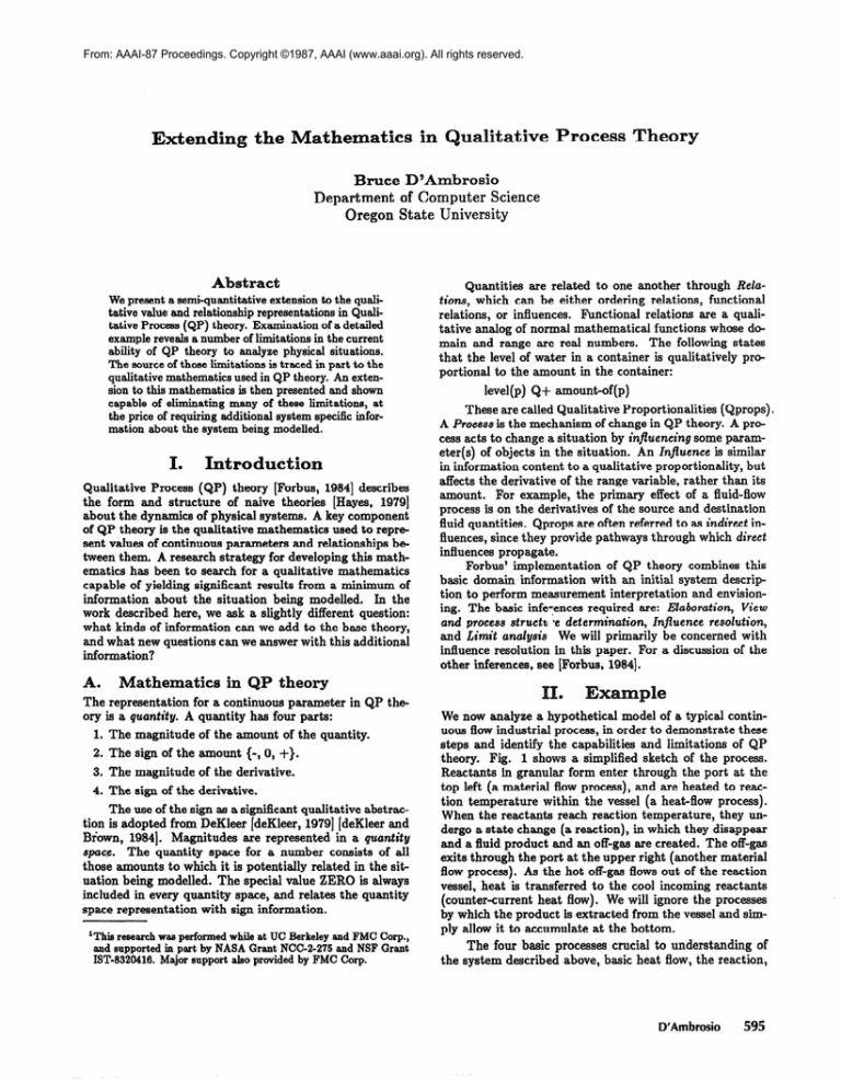
theory. Fig. 1 shows a simplified sketch of the process.
Reactants in granular form enter through the port at the
top left (a material flow process), and are heated to reaction temperature within the vessel (a heat-flow process).
When the reactants reach reaction temperature, they undergo a state change (a reaction), in which they disappear
and a fluid product and an off-gas are created. The off-gas
exits through the port at the upper right (another material
flow process). As the hot off-gas flows out of the reaction
vessel, heat is transferred to the cool incoming reactants
(counter-current heat flow). We will ignore the processes
by which the product is extracted from the vessel and simply allow it to accumulate at the bottom.
The four basic processes crucial to understanding of
the system described above, basic heat flow, the reaction,
D’Ambrosio
595
Offgas
-?
Reactants
0
0
A\\-
,roduct
Figure 1: Reaction Vessel
material flow, and counter-current heat flow, are described
in detail in [D’Ambrosio, 19861. Given a suitable initial
state description, the first two QP inferences identify three
possible states for the situation described, (1) that nothing
is happening, (2) that the only thing occurring is that the
reaction vessel is being heated, or (3) that all processes
are active. The state of interest is the one in which all
processes are active. Using the third basic QP deduction,
we can determine various facts about this state, such as:
e If the heat input is increasing, the off-gas generation
rate will be increasing also.
e If the incoming reactant temperature is decreasing,
the off-gas temp will be decreasing.
However, we cannot determine:
1. Is the product temperature increasing, decreasing, or
constant?
2. If the heat input is increasing, is the off-gas exit temperature increasing or decreasing?
3. If we increase the heat input a little, how much will
the generation rate increase?
4. If the available observations do not uniquely identify a
single state, which of the possible states is more likely?
These limitations are the result of ambiguity in the
conclusions derived using QP theory.
Ambiguity
in
theory
We identify two types of ambiguity in QP theory, Internal
and Ezternd ambiguity. Internal ambiguity occurs when
use of QP theory produces multiple descriptions of a single
physical situation. External ambiguity is the dual of this,
namely when a single QP theory description corresponds to
several possible physical situations which must be distinguished. Internal ambiguity is of two types. First, given a
situation description, there may be ambiguity about which
of several possible states a system is in (e.g., given a leaky
bucket with water pouring in, is the water level rising or
falling?). Second, given a specific state, there may be ambiguity about what state will follow it (e.g. - given a closed
container containing water, and a heat source heating the
container, will it explode?).
External ambiguity is the inability to determine, on a
scale meaningful to an external observer, the duration of a
situation, as well as the magnitude and intra-situation evolution of the parameters of the situation (e.g., how fast is
the water rising? How long before the container explodes?)
596
Engineering Problem Solving
1. Inability to resolve conflicting functional dependencies. This is caused by the weak representation for
functional form of dependencies, which captures only
the sign but no strength information.
2 Inability to order predicted state changes. This is
caused by lack of ordering information on change
rates, as well as lack of quantitative information on
the magnitude of change needed for state change.
Heat Source
I.
These ambiguities are the result of four fundamental limitations in QP theory representat ions and inference
mechanisms:
3 Inability to quantify, even approximately, parameters
significant to external observers during times between
major state transitions. This is caused by a weak
model of intrcGstate situation evolution. Time, quantity values, and functional dependencies are all represented qualitatively in QP theory.
4. Inability to represent non-boolean predicate and state
possibilities.
Solving these problems requires extending QP representations to capture more information about the system
being modelled. We have studied three classes of extensions: extensions to the quantity representations, the relationship representations, and the certainty representations.
Specifically, we have developed an extension to QP theory
which utilizes:
Belief functions certainty representations - these will
permit capture of partial or uncertain observational
data, and estimates of state likelihood.
Linguistic descriptions of influence sensitivities - to
reduce undecidability during influence resolution.
Linguistic characterizations of parameter values and
ordering relationships - to permit capture of partial
or uncertain observational data, and enable estimates
of the effects of adjustments to continuous control parameters.
These extensions reason at the appropriate level of detail for the kinds of control actions typically needed, draw
the needed distinctions, are computationally tractable, and
can reason with the imprecise or uncertain data typically
available. In this paper we concentrate on the second
of these extensions, linguistic influence sensitivities, and
present a way of annotationing the relationship representation in QP theory to reduce ambiguity. Discussion of
the integration of Dempster-Shafer belief functions with
QP theory and the underlying ATMS can be found in
[D’Ambrosio, 19871. Discussion of parameter value extensions can be found in [D’Ambrosio, 1986). See [Simmons,
19871for an alternate extended quantity representation.
IV.
Linguistic
ence
Sensitivities
The influence resolution rule used by Forbus states that
if opposite influences impinge on a single parameter, then
the net influence on the parameter is unknown. In order to reduce the number of situations in which conflicting
functional dependencies cannot be resolved, we extend
tern -lost
ie \
offgas temp/"+-$\
in furnace
;,"z;;,,";;P
43.
*
Q+-
offgas temp ~~;~~;;;;,
in furnace
Q+
a
Temp
Figure 2: Conflict Triangle
theory functional descriptions with a linguistic influence
sensitivity. Intuitively, this corresponds to distinguishing
between first order, second order, etc., dependencies. With
this extension we can now address the second question
unanswerable earlier: if we increase the heat input, will
the offgas temp increase or decrease?
Forbus claims that if actual data about relative magnitudes of the influences is available, it can be used to resolve
conflicts. We might attempt to achieve this by extending
direct and indirect influences with a strength parameter.
This is inadequate, however, for two reasons. First, the
overriding influence may not be local. Information may
have to be propagated through several influences before
reaching the parameter at which it is combined. Second,
various sources of strength information have varying scopes
of validity. In the following sections we first identify two
basic influence subgraphs responsible for the ambiguity in
our example, and argue that the ambiguity can be eliminated by annotating the subgraphs with influence sensitivity and adding additional situation parameters. We then
present extensions to the influence resolution algorithm for
utilising the sensitivity annotations, and finally describe a
control structure for managing acquisition and use of annotation information.
.
dentifying
internal
in influence graphs
(strqg)
causes
of conflict
We have identified two basic patterns of influences which
account for the ambiguity previously encountered. These
are the conflict triangle (Fig. 2) and the feedback loop
(Fig. 3). The reason, for example, that the change in offgas temp in the offtake cannot be resolved is that there
are two conflicting paths through which a single parameter
(offgas temp in the reaction vessel) affects the.target parameter. But the effect on temperature-lost is in this case
smaller than the direct effect on the offtake temp, and can
be ignored. We can indicate this by adding to the influence
arc an annotation indicating temp-lost in counter-current
heat flow is relatively insensitive to offgas temp in the furnace (Fig 2b).
Another ambiguity in the QP theory analysis of the
furnace is in the generation rate and associated variables.
One of the causes of this ambiguity is the set of influences
on Product temperature shown in Fig. 3. Since both the
Figure 3: Feedback Loops
generation rate and heat-flow rate are positive, the qualitative derivative of the product temperature is undecidable.
This network is similar to one Kuipers [Kuipers, 19861
identifies as introducing a new landmark value, not in the
original quantity space for the product temperature. This
new value represents an equilibrium value towards which
the temperature will tend. Recognition of the existence of
an equilibrium value permits resolution of the effects of the
conflicting influences on product temperature, depending
on the assumed ordering between the actual product temperature and the equilibrium value. analysis can be taken
one step further. Kuipers adds the equilibrium value to
the set of fixed points in the quantity space for the original variable. We, however, add it as a new parameter of the
model, subject to influences similar to those of the original quantity. Thus, we can represent and reason about
change in both the actual value and the equilibrium value
in response to active processes. For example, if the actual
temperature is only slightly sensitive to the heat-flow rate,
but the equilibrium temperature is very sensitive, then we
might conclude that the system will be slow in returning
to equilibrium once perturbed. The extended influence diagram for the feedback loop is shown in Fig 3b.
Sensitivity
mnotations
An influence is a partial function from the controlling variable to the controlled variable. In QP theory, computing
a value for a controlled variable takes place in two phases:
1. All of the individual influences on the controlled variable must be identified and the effect of each of these
must be computed.
2. The various effects must be combined to determine
the composite effect on the controlled variable.
This procedure relies on local propagation to perform
influence resolution. If local propagation is to carry the
burden of our extended influence resolution, then the prop
agated value must somehow be extended to represent the
sensitivity information. The value being propagated in
influence resolution is a quantity, and the representation
used in sign abstraction. Given our model of extended
influences as describing the normalised sensitivity of one
D’Ambrosio
597
variable to changes in another, we can simply extend the
quantity representation for the influence quantity and use
a discrete scale of influence magnitudes. We then represent the actual value as a fuzzy set over this value space,
to model the imprecision in the available sensitivity information. While this procedure is conceptually simple,
the question arises of how an appropriate discretization
for this normalised change value, henceforth referred to as
influence, can be determined.
If we start with an n-level influence discretization and
an m-level sensitivity discretization, then after k influence
propagation steps we seemingly might need an nmk discretization to avoid information loss. This worst case complexity can be substantially reduced, however, by the following four observations:
member of the value sets for both input values, or if it is
a member of the value set for one input, and a weaker element of the same sign is a member of the value set for the
other input. Also, an element of the discretization may be
an element of the result set under two conditions. First, if
it is a member of the value set of one input, and a element
of the same magnitude but opposite sign is a member of
the value set for the other input. Second, if an element of
the same sign but greater magnitude is a member of one
value set, and an element of the opposite sign and greater
magnitude is a member of the other value set:
PI”(i)
3. Rather than annotating all influences in a graph, we
will only annotate those necessary to disambiguate parameters of interest in a specific query.
4. The basic fuzzy relational influence algorithm can be
designed so that failure to maintain a fully detailed
discretization only increases the ambiguity of the result, rather than produce incorrect results.
Given this, we model sensitivity annotations as p&
rameters of a standard fuzzy relational influence algorithm
[Zadeh, 19731. We choose a fuzzy representation to allow
simple modelling of the imprecision of these annotations2.
We next detail the algorithms used to compute the consequences of this fuzzy algorithm.
1.
Computing individual influences
An influence of the form:
(Influenced-variable Q+/- Influencing-variable,
Sensitivity)
v(/.m(i)
Sk)
=
8dgn(
cj
* Sk)
*
(abs(Cj
Combining influences
Sensitivity annotations provide us with a means of
estimating influence magnitudes, which are directly comparable. Below we show an algorithm for computing the
combined effect of two influences. A rough translation is
that an element is definitely a member of the set of possible values for the combined influence if that element is a
2The underlying model is of a set of independent, linear influences.
Fuzzy eet models of sensitivities permit us to allow for the inaccuracies of this model.
598
Engineering Problem Solving
A
unknown))
C.
Annotation
Mana
In examining the sources of ambiguity in the reaction vessel example, we note that many of the annotations which
could resolve the ambiguities are not universally valid. In
fact, we identify four levels of validity for an annotation.
These validity levels are determined primarily by opportunities in the implementation:
1. An annotation is universally valid when it can.be incorporated directly into a view or process description,
and correctly describes the functioning of a particular
influence in all situations in which an instance of the
view or process participates. These are rare.
2.
An annotation is scenario valid when it correctly describes the operation of a particular influence in a
particular view or process instance, for all qualitative
states in which the instance is active. Product temperature annotations in the example are an instance
of this annotation type.
3.
An annotation is state valid when it correctly describes the operation of a particular influence in a
view or process instance, only for a defined subset of
the qualitative states of a system.
4.
Annotation is query valid when it correctly describes
the operation of a particular influence in a view or process instance, only for a particular query. The conflict
triangle annotation for determining off-gas temperature in the offtake is an example of this type of annotation.
* Sk)““)
2.
pI,z(k)
Subsrcipts i, j, and k are assumed to be 0 for no influence, increasing positive for positive influence elements,
and increasing negative for increasing negative influence
elements (e.g., -3, -2, -1, 0, 1, 2, 3 for a seven element discrete scale, with -3 the strongest negative inlluence). The
above is only half of the formula actually used. The actual
relation is symmetrical in the two influences Iv1 and Iv2.
C.S
&I,C,S(cj,
A /4clluz(--i)
~unknown)
V(Vj,j>i Vk,k<-i (hrvl(j) A
is taken to specify a fuzzy relation between three amounts:
C, the amount of the influencing variable; S, the amount
of the influence sensitivity; and Iv, the amount of the influence on the influenced variable. The value of Iv can be
computed as follows:
Iv = C(min(lcc,CcsrClq)lQl,c,s(C,
S))
(PZ"l(i')A Clrvz(i))
V(Vj,ljl<lil(ClIul(i)
APIv2(.i)))
1. We are only interested in the result at a resolution
equivalent to the original n-level discretization.
2. Additional detail is only relevant when two annotated
influences are being combined, to aid in influence resolution if they conflict.
=
The first type of annotation can simply be part of
the basic view or process detiition. The other three are
added to the QP description of a scenario as needed during
problem solving. A four step algorithm extends the basic
QP theory influence resolution algorithm:
1. Execute the basic influence resolution.
2. Check results for ambiguities in parameter values of
interest. If all’interesting parameter values are determined uniquely, then problem solving is complete.
[Zadeh, 19731Lofti A. Zadeh. Outline of a New Approach
to the Analysis of Complex Systems. In IEEE Tkansactions of Systems, Man, and Cybernetics, 3(1):28-44,
1973.
3. Otherwise, search the influence graph for instances of
ambiguity causing subgraphs. If one is found, and the
parameter for which it might create an ambiguity is
ambiguous, then annotate the subgraph with influence
sensitivity information if available.
4. Re-execute the basic influence resolution algorithm on
the now annotated graph.
This algorithm assumes the extended QP reasoner is
embedded in a larger system which has or can obtain the
necessary problem specific information to resolve ambiguities. It provides a problem directed way of selecting aspects
of the larger system’s problem specific knowledge relevant
to the query being processed.
.
Summary
We have described an extension to QP theory which increases the precision of results available, and still retains
the inherent advantages of qualitative modelling. This
extension derives its power from influence sensitivity annotations, and a fuzzy mathematical model of influences
which permits propagation of the effects of these sensitivities throughout the influence chart.
eferences
[D’Ambrosio, 1986] Bruce D’Ambrosio.
Qualitative Process Theory using Linguistic
Variables.
Phd thesis,
University of California, Berkeley, 1986.
[D’Ambrosio, 19871 Bruce D’Ambrosio.
Truth Maintenance with Numeric Certainty Estimates. In Proceedings Third Conference on AI Applications, pages 244249, Kissimmee, Florida, Computer Society of the
IEEE, February, 1987.
[deKleer, 19791Johan deKleer.
Causal and Teleological
Reasoning in Circuit Recognition.
Technical Report AI-TR-529, Artificial Intelligence Laboratory,
Massachusetts Institute of Technology, October 1979.
[deKleer and Brown, 19841 Johan deKleer and John Brown.
A Qualitative Physics Based on Confluences. Artificial Intelligence, 24( 1-3) :7-83, December 1984.
[Forbus, 19841Kenneth Forbus. Qualitative Process Theory Phd Thesis, Massechusetts Institute of Technology, July, 1984.
[Hayes, 19791Patrick J. Bayes. The Naive Physics ManiAge.,
festo. IIn Expert Systems in the Micro-Electronic
D. Michie, (editor), Edinburgh University Press, Edinburgh, Scotland, 1979.
[Kuipers, 1986] Benjamin J. Kuipers. Qualitative Simulation. Artificial Intelligence, 29(3):289-338, September
1986.
Commonsense Arit h[Simmons, 19871 Reid Simmons.
metic Reasoning. In Proceedings AAAI-86, pages P18124; Philadelphia, Pennsylvania, American Association for Artificial Intelligence, August, 1986.
D’Am brosio
599
