From: AAAI-87 Proceedings. Copyright ©1987, AAAI (www.aaai.org). All rights reserved.
Learning to Control a
Dynamic
Physical System
Margaret
E. Connell
Paul E. Utgoff
Department
University
of Computer
and Information
Science
of Massachusetts,
Amherst,
MA 01003
Abstract
This paper presents an approach to learning to control
a dynamic physical system. The approach has been implemented in a program named CART, and applied to a simple
physical system studied previously
by several researchers.
Experiments
illustrate
that a control method is learned in
a.bout 16 trials, an improvement
over previous learning programs.
I.
research perspective,
a control problem presents a unique
challenge
for learning methods.
First, the dynamics of a
physical system impose the constraint
that successor states
cannot be chosen arbitrarily.
This means that anticipation
and prediction
of future states become critical.
Second,
training information
is often delayed, making credit assignment for individual
actions difficult.
The approach taken here is to investigate
a control problem that has been studied previously by connectionists
and
control theorists.
In general, one would like to either remove assumptions
or exchange them for simpler or cheaper
ones. The primary goal of the work reported here is to remove a certain collection of starting assumptions
that have
been adopted in previous work.
This requires a different
knowledge representation
and a new action selection mechanism.
The Cart-Pole
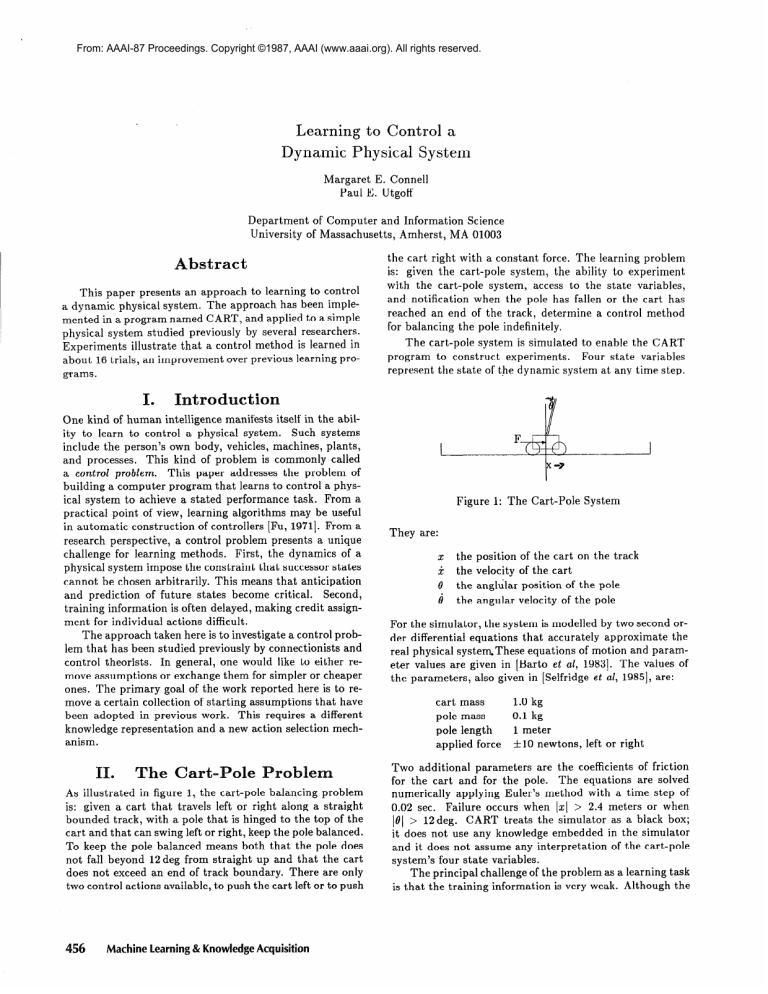
As illustrated
in figure 1, the cart-pole
balancing
problem
is: given a cart that travels left or right along a straight
bounded track, with a pole that is hinged to the top of the
cart and that can swing left or right, keep the pole balanced.
To keep the pole balanced means both that the pole does
not fall beyond 12 deg from straight
up and that the cart
does not exceed an end of track boundary.
There are only
two control actions available, to push the cart left or to push
456
with the cart-pole
system,
access to the state variables,
and notification
when the pole has fallen or the cart has
reached an end of the track, determine
a control method
for balancing
the pole indefinitely.
The cart-pole
system is simulated to enable the CART
program
to construct
experiments.
Four state variables
represent the state of the dynamic system at any time step.
Introduction
One kind of human intelligence
manifests itself in the ability to learn to control a physical system.
Such systems
include the person’s own body, vehicles, machines, plants,
and processes.
This kind of problem is commonly
called
a control problem.
This paper addresses
the problem of
building a computer program that learns to control a physical system to achieve a stated performance
task. From a
practical
point of view, learning algorithms
may be useful
in automatic
construction
of controllers
[Fu, 19711. From a
HI.
the cart right with a constant force. The learning problem
is: given the cart-pole
system,
the ability to experiment
Machine learning & Knowledge Acquisition
Figure
They
For
der
real
eter
the
1: The
Cart-Pole
System
are:
x
the position
of the cart on the track
i
the velocity
of the cart
8
the anglular
i
the angular
position
velocity
of the pole
of the pole
the simulator,
the system is modelled by two second ordifferential
equations
that accurately
approximate
the
physical system.These
equations of motion and paramvalues are given in [Barto et al, 19831. The values of
parameters,
also given in [Selfridge et al, 19851, are:
cart
mass
pole mass
1.0 kg
pole length
0.1 kg
1 meter
applied
f10
force
newtons,
left or right
Two additional
parameters
are the coefficients
of friction
for the cart and for the pole.
The equations
are solved
numerically
applying Euler’s method with a time step of
Failure occurs when 1x1 > 2.4 meters or when
0.02 sec.
101 > 12deg.
CART treats the simulator
as a black box;
it does not use any knowledge embedded in the simulator
and it does not assume any interpretation
of the cart-pole
system’s four state variables.
The principal challenge of the problem as a learning task
is that the training information
is very weak. Although the
learning
during
system
stores
an experiment
the history
at balancing,
of the states
encountered
it is only told when the
pole has actually
fallen, i.e. the pole has swung beyond
l2deg
from straight
up or when the cart has reached an
end of the track. Due to the dynamics of the cart and pole,
and the limits imposed by the performance
task, the cartpole system can be in a state from which no sequence of
control forces will keep the pole from falling or keep the
cart from reaching
an end of the track.
Such a state is
called “doomed”. -The learning problem does not assume
the existence
of a critic that immediately
identifies good
versus bad actions.
Furthermore,
even if one were able to
characterize
a state as doomed or not, it is not obvious how
to avoid doomed states using the available control actions.
.
elated
OSlS
The problem was investigated
in 1964 by Widrow and Smith
[Widrow & Smith, 19641. It has been studied by Michie and
Chambers
(Michie & Chambers,
19681, and also Anderson,
Barto, Selfridge, and Sutton /Anderson, 1986; Barto et al,
1983; Selfridge et al, 19851. In all of these cases, the learning problem has been to construct
a program that learns
to keep the pole balanced.
Michie and Chambers
[Michie & Chambers,
19681 built
a program named BOXES-that
learned to balance the pole.
They mapped each of the four state variables of the cartpole into a discrete value, depending on predefined ranges
for each variable.
The 5 ranges for the cart, 3 for the cart
velocity, 5 for the pole, and 3 for the angular velocity produced a total of 225 distinct regions.
For each action and
region, the average time until failure was updated from the
experience
of each trial. For a given region, BOXES chooses
the action with the higher average time until failure.
The
program required about 600 trials to learn to balance the
pole for 72,000 time steps (each .05 set).
Michie and Chambers point out that the choice of ranges
for the cart variables
(the size of the boxes) is critical
to
the success of the BOXES
program.
A poor choice of
ranges makes the system unable to learn to balance the
pole. Hence, choosing ranges that permit learning to balance the pole is a necessary step for this approach.
Choosing these ranges requires experimentation
or analysis and
should therefore
be considered
part of the learning problem. Dividing the state space into regions is exactly the set
of starting
assumptions
that were eliminated
in the CART
program.
Barto, Sutton and Anderson[Barto
et al, 19831 improved
on the results of Michie and Chambers
by designing two
neuronlike
adaptive elements,
that were used to solve the
same balancing
task. They also employed a division of the
state space into predefined distinct regions. The action with
the higher probability
of keeping the pole balanced was the
one chosen in each region. The system was able to balance
the pole over 60,000 time steps before completing
100 trials. On the average by the 75th trial, the pole remained
balanced over 8000 time steps (each .02 set).
More recently, Anderson[Anderson,
19861 devised a connectionist
system to learn to balance the pole. His system
trains two predefined
two-layer networks.
One learns an
evaluation
function,
and the other
learns
an action
func-
tion over the state-space.
Learning occurs by successively
adjusting
both the weights of the evaluation
and action
networks.
His system has the advantage that it is not necessary to provide well-chosen
boxes ahead of time. This is
achieved at considerable
cost in terms of performance;
his
system takes an average of 10,000 trials to learn to balance
the pole for approximately
7000 steps.
rogram
This section presents the CART program, which learns to
balance the cart-pole system indefinitely
after about 16 trials. The program is explained in terms of a classic learning
model [Smith et al, 19771, which consists of four components considered
necessary
for a learning system:
a Problem Generator,
a Performance
Element,
a Critic,
and a
Learning Element.
The Problem
Generator
initializes
a new experiment,
called a trial. The Performance
Element applies a left or
right control force at each time step, attempting
to balance
the pole indefinitely.
The Critic labels some of the states
from the trial as desirable
(value 1) or undesirable
(value
-1). Based on input from the Critic, the Learning Element
updates its concept of the degree of desirability
of a state.
Because
the Performance
Element
decides which control
action to apply, based on its estimate of whether an action
will lead to a more desirable state, learning to estimate the
degree of desirability
of a state improves performance.
The cart program learns and employs the concept of the
degree of desirability
of a cart-pole
state.
A concept that
represents
degree of desirability
is fundamentally
different
from one that represents
only desirable or not desirable.
The degree of desirability
of a cart-pole state is represented
by an explicit function of the 4 state variables of the cartpole system.
The function is modified by the Learning Element, as described below. For each trial at balancing,
the
function remains fixed. The degree of desirability
of a cartpole state is computed
using Shepard’s function
[Barnhill,
1977; Schumaker,
19761, which interpolates
from known desirable and undesirable
states that were supplied previously
by the Critic.
Shepard’s
interpolation
method was chosen
because all interpolated
values fall smoothly
between the
maximum and minimum
observed values, making it well
suited to the cart-pole
problem.
’
Given the n points zi = (zr,;, x2,;, xs,i, . . . , x,,+) in mdimensional
space, with known values f(zi) = Fi for i =
1 . . . n, Shepard’s
interpolating
function
is:
where
j=l,j#i
(x1
-
X*,j)2
+
(X2
-
X2,j)2
+
e ms +
(2,
-
X,,j)2,
the distance from z to a known point zj, and p > 0. p = 2
was used at all times based on the recommendation
of Schumaker [Schumaker,
1976). Note that the known desirable
Connell and Utgoff
457
and undesirable
states are retained,
that their values are
preserved
by the interpolating
function,
and that the degree of desirability
of any state is determined solely by these
known examples
(states).
It can be seen from the function that designated
desir-
of the same action would take the system.
The gradient
of the interpolating
function, evaluating
desirability,
is a 4dimensional
vector that points in the direction of maximum
increase of the function at a point (state).
able and undesirable
states that .are near to a given cartpole state have greater
influence on the function’s
value
than those at a distance.
This is because the weights, wi,
associated
with the near sta\es are greater.
Ideally, the action
the action that would
state that more nearly
Without
the ability to
sary to use a decision
A.
each successive state the angle between the gradient at the
point and the extended vector is computed
by taking the
Problem
Generator
selection
mechanism
would choose
cause the system to move to the
lies in the direction of the gradient.
predict successor states, it is necesstrategy
that is less than ideal. At
The task of the Problem Generator
is to initialize the cartpole system so that an experimental
trial at balancing can
be performed.
The cart-pole
system is initialized with the
inner product
of the two vectors.
If the angle decreases
(because
direction
and gradient
are better aligned),
then
the decision is to repeat the same action.
cart near the center of the track and with the pole nearly
upright.
These values for the cart and the pole are selected
to vary a small random amount from exactly centered and
exactly vertical.
The initial cart velocity and pole angular
velocity are set to 0. This initialization
procedure places the
cart-pole
system in a state from which indefinite balancing
is possible.
This fact is used by the Critic.
The algorithm
is illustrated
in figure 2. The two control
actions are labelled L and R. Since /a3 < /a2 (the angle
B.
Performance
Element
The task of the Performance
Element is to choose a control
action (push left or push right) at each time step so that
The decision procedure
selects an acthe pole balances.
tion which is expected to lead to a more desirable successor
state.
The dynamics of the system and the limited choice
;Z is the extended vector
Figure
2: Continue
Same
Action
at ss
of control action impose the fundamental
constraint
that it
is not possible to move to an arbitrary
successor state. The
action selection problem is further compounded because the
Performance
Element
does not know the dynamics of the
system or the effect of a control action.
At every step the Performance
Element decides whether
to repeat the same action or to change to the other. If, by
continuing with an action, it is estimated
that the cart-pole
system will move to a more desired state, then the same
action is repeated.
Otherwise,
the other action is selected.
To facilitate
the decision, two vectors are computed at each
point, the gradient and the extended vector. The direction
of the extended vector, defined by continuing from the state
in the same direction as the system is already travelling,
is a
useful estimate of the direction in which another application
l A. Barto has pointed out that Shepard’s method is a special case
of the method of potential functions.[Duda & Hart, 197.71
458
Machine learning & Knowledge Acquisition
between w’~and grad3 is less than the angle between V> and
grud2), the system is estimated
to be moving in a desirable
direction
and the choice of action at s3 will again be L.
If /a3 > /a2 then the continuation
of the last action is
estimated
to lead away from desirability;
as a result, the
choice of action at s3 will change to R.
cc.
Critic
The Critic must supply information
that makes it possible
for the Learning
Element
to improve its abilility
to estimate the degree of desirability
of all cart-pole
states.
This
is done by labeling certain states in the trial as desirable
or undesirable.
Choosing
a particular
cart-pole
state and
determining
whether it is desirable (value 1) or undesirable
(value -1) is done in three ways.
First, as described above, the cart-pole system is initialized to a state from which indefinite balancing is possible.
The first state in each trial could be labelled as a desirable state.
As a shortcut,
the CART program initializes
the learning process by labelling
the state with the pole
straight-up,
the cart centered,
and 0 velocities
a desirable
point. It is the prototypical
start state.
Second,
when the pole falls, an undesirable
state has
been reached.
The Critic labels the state immediately
preceeding the failure as undesirable,
unless the degree of desirability
of the state is already less than -0.98.
Third, when the cart-pole
system has balanced longer
than 100 time steps, it is inferred that some of the states
were desirable.
This is based on the fact that a random sequence of control actions keeps the pole balanced for about
20 time steps. When a trial has ended and has lasted longer
than 100 steps, the Critic searches the sequence of states
for one that it will label as desirable.
The algorithm
is:
backup 50 steps from the failure point; then keep backing
up until a point is found at which 3 or more of the cart
variables
are decreasing
in magnitude;
label that point as
desirable.
This algorithm is based on the assumption
that a
state which occurs 50 time steps before failure is in a good
position
if it is a state from which the system is moving
toward the prototypical
start state (the point from which
indefinite
balancing
is possible).
These numeric parameters
(100, 50, 3) were determined
empirically
through experimentation
with the system.
An
improvement
would be for a learning system to do this ex-
perimentation
and determine
these
parameters
itself.
Ex-
perience suggests that these parameters
may be a function
of the system performance
prior to learning (e.g. The first
parameter
could be 5 times the length of a random trial.)
.
Learning
Element
The task of the Learning
Element
is to improve its accuracy in estimating
the desirability
of a cart-pole state. The
Critic provides specific training instances
to the Learning
Element.
A training instance is a 4-dimensional
point in
cart-pole
state space that has been labelled as desirable (1)
or undesirable
(-1). The Learning
Element needs to generalize, so that it can estimate the desirability
of points that
it has not seen as training instances.
A function defined by Shepard’s
method requires a set
of points from which to interpolate.
Learning is therefore
quite simple;
add a new point (training
instance),
along
with its label (+I or -l), to a list of all observed training instances.
Because the speed of Shepard’s
formula is
a function of the number of training instances
(to evaluate
the formula at any point the distance to every training instance must be calculated),
it is important
that the Critic
deliver a small number of well chosen training instances to
the Learning Element.
For the cart-pole problem, not many
observed states are necessary for developing a good interpolation function and the Critic chooses the points well.
A version of Shepard’s
method was implemented
that
updates the symbolic formula incrementally.
This is more
efficient than rederiving the formula with each new training
instance.
With each new point, .zk = (~i,k,x~,k,. . . ,~~,k),
only one new explicit distance formula is derived,
dk
=
j/(x1
-
one more term
xl,k)2
+
(x2
-
x2,k)2
+
is added to the product
**.
+
(%I.
-
%,k)2,
of the existing
dis-
tances and one new product of distances is evaluated.
It is helpful to view the desirabilty
of a cart-pole state as
the height of a surface in S-dimensional
space. The first four
dimensions of a point on the surface designate the cart-pole
state, and the fifth, its degree of desirability.
The surface
is changed after each trial as new points are supplied to
the Learning Element.
This means that subsequent
performance is also likely to change.
As a result, in successive
trials different regions of the cart-pole
state space are ex-
RUN NUMBER
1
T
1
27
R
2
79
167
Al
4”
9
Lj
5
242
6
171
N
7
9
195
u
8
M’9
6G4
B
lo
5000
E
11
R
12
13
14
j 15
16
*intll
Figure
3
29
9
2
25
9
179
9
81
224
104
19
229
84
139
10
183
582
5000
136
240
24
274
4
12
163
154
55
172
281
5000
3: Number
of Steps
6
13
9
5
26
199
88
9
79
323
11
173
24
*11
10000
252
*11
150
*11
*11
12
382
per Trial
the cart-pole
system developes a pattern of behavior
repeats itself and is indicative of indefinite balancing.
that
The CART
program was run 14 times.
In every case, it
learned to balance the pole. Furthermore,
the system behavior fell into a distinct
pattern
every time, suggesting
that additional
runs would not turn up anything new. As
seen from a sampling
of the runs in figure 3, the CART
system learned the control task in 16 or fewer trials, sometimes in as few as 9 trials. Of the runs tried, 10 were halted
at 5000 time steps and 3 runs were halted at 10000 time
steps.
The final run was halted at 70000 time steps, the
equivalent
of 25 minutes of balancing.
Figure 4 illustrates
the cyclic pattern behavior that developed.
As the pole falls in one direction,
the cart is
pushed in the same direction to arrest the falling pole. This
continues
necessarily
until the pole has sufficient velocity that
start to move in the opposite direction.
it will
When
X
plored.
New trials force the system to learn nonrepetitive
and useful information.
On the first trial the pole typically
falls while the cart remains near the track’s center.
The
resulting
surface slopes down from the center toward the
undesirable
point.
In the next trial the choice of actions
will force the cart-pole
system to move away from failure
and the pole will fall in the opposite direction.
After a few
trials the cart will move out from the center of the track
where the values on the surface are greater.
When the cart
reaches the track boundary
in one direction,
the surface
will slope down toward that boundary
forcing the cart to
move in the opposite direction during the subsequent
trial.
As the learned surface improves, balancing
time increases.
Soon the number of steps exceeds 100 and a desirable point
other than the center is determined.
After 10 to 15 trials,
Figure
4: A Typical
Run in 2-Dimensions
Connell and Utgoff
459
this happens the cart is pushed in the opposite
direction
to stop the falling pole again. This balancing
activity also
keeps the cart from creeping toward an end of the track.
The pattern depicted in the figure shows activity along the
right diagonal, which corresponds
to the behavior described
above. Balancing occurs when a push decreases the velocity
of both the cart and the pole. This will happen only when
the cart and the pole are moving in opposite directions.
An
illustration
usgng run 3 is shoyn in figure 4.
x-axis
position
of the cart
e-axis
-n
position
of the pole in radians
+”
a desirable
+O
arrows
show the repeated
points
states
Additional
an undesirable,state
state
the given central
showed
on nth trial
on nth trial
the system
learns
under different conditions.
In every case described below
balancing
occurred
in !ess than 18 trials.
The variations
ma-de in these experiments
were the same as those made
et al, 19851.
One experiment
was
by Selfridge
[Selfridge
to increase the original mass of the pole by a factor of 10.
Other experiments
were to reduce the mass and length of
the pole to two-thirds
of the original values, to reduce the
total length of the track to 2 meters from 4.8 meters, and
to apply unequal
tons).
forces
left (12 newtons)
and right
(8 new-
The CART program demonstrates
an algorithm
for learning a. control method to satisfy a particular
performance
task. An important
objective
was to build a program that
does not depend on a predefined partition
of a continuous
state space into discrete regions. This was accomplished
by
representing
the degree of desirability
of a state by a continuous interpolating
function of the state variables.
This
representation
necessitated
a new action selection mechanism that makes use of the current state and the learned
concept of the degree of desirability
of the system state.
More work is needed to explore the generality
of the
CART system.
The system is general to the extent that it
does not depend on an interpretation
of the state variables;
it simply learns to select control actions so that failure is
avoided.
The CART program does .take advantage of the
fact that the system is initialized
to a state from which
indefinite
balancing
is possible.
It also takes advantage of
the continuity
of the cart-pole
system and the smooth behavior of the function
representing
degree of desirability.
An important
characteristic
of the learning problem is that
there is no criticism
at each time step. Reliable
criticism
is available only when the pole falls.
It was necessary
to
construct
a Critic that was able to classify cart-pole
states
as desirable or undesirable.
Further work is needed to explore the extent to which the Critic algorithm
depends on
characteristics
of the cart-pole
problem.
460
Machine learning & Knowledge Acquisition
19861 Anderson,
C. W.
Learning
and Problem
Connection&
Systems
UniPh.D.
Dissertation.
COINS
86-50: Amherst,MA.
1986.
[Barnhill,
19771 Barnhill,
R. E. “Representation
and
proximation
of Surfaces”
Mathematical
Software
Academic Press, 1977.
point
pattern
that
eferences
Solving with Multilayer
versity
of Massachusetts
TECHNICAL
REPORT
at 50 step intervals
experiments
Andy Barto
generously
provided
his cart-pole
simulator
and was a valuable source for discussion and criticism.
We
thank Sharad Saxena, Chuck Anderson, and Peter Heitman
for the helpful discussions
and comments.
The reviewers
made several useful suggestions.
[Anderson,
in meters
desirable
cknowledgements
ApIII,
A. B., Sutton,
R. S. and An(Barto et al, 19831 Barto,
derson,
C. W. “Neuronlike
Adaptive
Elements
that
can Solve Difficult Learning Control Problems.”
IEEE
Trans. on Systems,
Man and Cybernetics,13
no 5.,
1983.
Duda & Hart, 19731 Duda, R. and Hart, P. Pattern
sification and Scene Analysis, Wiley, N.Y. 1973.
Fu, 19711 Fu, K. S. Pattern and Machine
Press, New York-London,
1971.
Clas-
Learning Plenum
Michie & Chambers,
19681 Michie D. and Chambers
R.,
“Boxes An Experiment
in Adaptive
Control”,
in Machine Intelligence
z?, E.Dale and D. Michie Eds. Oliver
and Boyd, Edinburgh,
1968.
[Schumaker,
19761 Schumaker,
L. L. “Fitting
Surfaces
to
Scattered
Data” Approximation
Theory II. Academic
Press, 1976.
[Selfridge et al, 19851 Selfridge
0. G., Sutton
R. S., and
Barto A. G. “Training
and Tracking
in Robotics”
in
Proceedings
of the 9th International
Joint Conference
on Artificial Intelligence, Los Angeles, CA. 1985.
Smith et al, 1977) Smith R. G., Mitchell T. M., Chestek R.
and Buchanan
B. G. “A Model For Learning Systems”
in Proceedings of the 5th International Joint Conference
on Artificial Intelligence Cambridge
MA. 1977.
Widrow & Smith, 1964) Widrow,
B. and Smith
F. W.
“Pattern-recognizing
Control
Systems”
in Computer
and Information
Sciences, J. Tou and R. Wilcox Eds.
Clever Hume Press, 1964.