KSU Willie in the AAAI 2007 Semantic Vision Challenge
Dr David A Gustafson, Michael Marlen, Aaron Chavez, and Andrew King
Kansas State University, Computing and Information Sciences
234 Nichols Hall, Manhattan, KS 66506
{ dag, mchav, msm6666, aking }@ksu.edu
autonomously on images downloaded from the internet.
The resulting trained classifiers were used to identify the
objects in the environment. The effectiveness of the
classifiers on the training set were used to determine which
classifier or set of classifiers was used for each object in
the environment.
Abstract
Kansas State University competed in both the robot division
and the software division of the AAAI 2007 Semantic
Vision Challenge. The team used a Pioneer P3AT robot,
scalable client/server software architecture, path-planning
code, and a set of image classifiers that autonomously
trained on images downloaded from the internet. The team
succeeded in identifying multiple objects in the
environment.
Marlen Perceptual Model
The Marlen Perceptual Model provides a unique way of
looking at objects. MPM is based on pairs of colors. The
restriction on the pair is that the first color must be
adjacent to the second color and that the colors are sorted
from least to greatest.
Introduction
The Kansas State University entry into the AAAI 2007
Semantic Vision Challenge consisted of a Pioneer P3AT
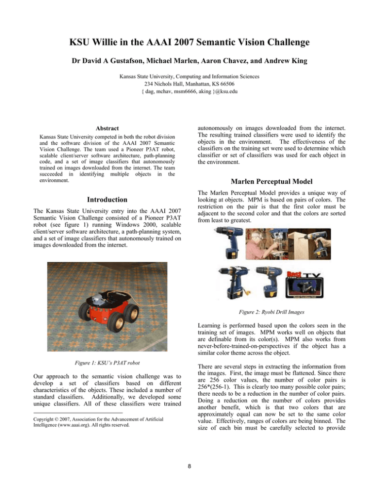
robot (see figure 1) running Windows 2000, scalable
client/server software architecture, a path-planning system,
and a set of image classifiers that autonomously trained on
images downloaded from the internet.
Figure 2: Ryobi Drill Images
Learning is performed based upon the colors seen in the
training set of images. MPM works well on objects that
are definable from its color(s). MPM also works from
never-before-trained-on-perspectives if the object has a
similar color theme across the object.
Figure 1: KSU’s P3AT robot
There are several steps in extracting the information from
the images. First, the image must be flattened. Since there
are 256 color values, the number of color pairs is
256*(256-1). This is clearly too many possible color pairs;
there needs to be a reduction in the number of color pairs.
Doing a reduction on the number of colors provides
another benefit, which is that two colors that are
approximately equal can now be set to the same color
value. Effectively, ranges of colors are being binned. The
size of each bin must be carefully selected to provide
Our approach to the semantic vision challenge was to
develop a set of classifiers based on different
characteristics of the objects. These included a number of
standard classifiers. Additionally, we developed some
unique classifiers. All of these classifiers were trained
Copyright © 2007, Association for the Advancement of Artificial
Intelligence (www.aaai.org). All rights reserved.
8
enough distinctiveness between objects. The value used in
the contest was 51 values per bin. This provided a
manageable set of bins. All the pixels in each image were
put into the bins and the resultant picture is a flattened
image which has lost minimal defining characteristics.
The results for the Ryobi Drill were exceptional (not
shown). All pictures of the Ryobi Drill were classified as
containing a Ryobi Drill. None of the images that were not
classified as Ryobi Drill by the human was labeled
incorrectly. Thus, the error rate was 0% for misclassifying
the Ryobi Drill.
Figure 3: BookImages
Figures 2 and 3 shows some of the images that were
successfully downloaded from Google’s image search.
The images in figure 2 became the positive training
examples for the Ryobi Drill and the images in figure 3
became the positive training images for the book
“Probabilistic Robotics” respectively. The set of images in
Figure 3 also acts as the negative training set for the Ryobi
Drill. The set of images in Figure 2 act as the negative
training set for the book “Probabilistic Robotics”.
Additional images were included in the negative training
sets from searches on Horizon, Grass, Desk, Empty Room,
Table, Whiteboard, and Soccer Field. None of the negative
training images are shown.
After extracting and learning the relevant pairs of color for
each respective object a test set was given to MPM to
determine the ability to detect the object in an image.
Figure 4 shows both examples of a Ryobi Drill as well as
the book “Probabilistic Robotics”. Both objects are placed
into the test set to see if MPM is able to distinguish
between the two objects. The images listed in the below
figures are just a part of the complete set.
It turns out that MPM works for these two particular
objects because the pair of colors that are selected turn out
to be unique to the object. The bounding boxes for some
of the images in the test set are shown in Figure 5. The
green box bounds two distinct regions that neighbor each
other that indicate the book “Probabilistic Robotics”. As
seen in the 4th and 6th images in figure 5, false positives
have been detected.
Figure 4: Images in Test Set
The running time of the algorithm is also extremely low. It
takes approximately 21 seconds to train on 60 images and
to test if twenty images contain one of the two particular
objects. For every 45 more images that are added the
algorithm running time increases by approximately 14-15
seconds running on a 2.6 GHz machine.
9
The MPM, given a strong set of training images, performs
well on objects where the object color patterns are a
defining attribute to the object. To be a strong training set
of images, there are two criteria. First, the training images
must have a similar color theme (high correlation between
color patterns) for the positive training set and, second, the
negative training set examples must contain background
information contained within the positive training set..
generating a set or bag of features that are highly relevant
to the object class. Once this bag has been collected
objects in the image are detected and located by the
amount of relevant features for the class in the image.
Bag collection works by collecting all features present in
the positive training set. This collection is pared down by
comparing each feature in the set with every other feature
using Euclidean distance. If the distance is below a certain
threshold the comparison is considered a match and the
duplicate is discarded.
Next an array of integers is created equal in size to the
number of unique descriptors in the positive feature set.
This table is used to tally the relevance of the feature in
question. Each feature in the negative collection is
compared with each feature in the positive set. Each time a
match occurs then that feature’s tally is decreased. The
original full feature set is then compared with the pared
feature set. Each time a match occurs that features tally is
increased.
The final bag is selected by taking all features whose tally
is above a certain threshold.
Classification with this bag is straightforward. A list of
features from the image being classified is compared with
the classifier bag. If matches occur the number of matches
is recorded for that image as a potential match for that
object class. The location of the features is used to
generate a bounding box that localizes the detected object.
Our approach can use any feature that can be compared
using Euclidean distance. We used SURF(Bay,Tuytelaars,
and VanGool) a SIFT-like descriptor and feature detector.
Geometric Feature Descriptor
The geometric descriptor attempts to recognize objects
using basic shapes/outlines.
Initially, an image
segmentation algorithm divides the picture into regions.
We must then find outlines of potential objects by finding
the edges between “foreground” and background”. If a
region is sufficiently large, it is labeled as background.
Then, we need only locate the regions directly adjacent to
the background.
Figure 5: Bounding Boxes
Once the regions of interest are located, we must classify
them. We first find the prominent lines in the image with a
Hough transform. Then, we convert them to line segments.
Next we group each pair of lines and convert them into a
descriptor.
So, each descriptor describes one pair of line segments.
The parameters for the descriptor are ratio, orientation,
angle, and distance. The ratio describes the length of the
Relevant Feature Bagging
One of our primary concerns when developing our feature
descriptor based classifier is the speed of both the classifier
learning and that classification. Our solution involves
10
longer segment, relative to the length of the shorter. The
orientation describes the angle of the longer segment
relative to the image itself. The angle describes the angle
between the two segments. The distance describes an
approximation of the distance between the two segments.
to process pictures in less than one second, allowing realtime identification of the objects.
Conclusions
One of our primary concerns when developing our feature
descriptor based classifier is the speed of both the classifier
learning and that classification. Our solution involves
generating a set or bag of features that are highly relevant
to the object class. Once this bag has been collected
objects in the image are detected and located by the
amount of relevant features for the class in the image.
Classification with this bag is straightforward. A list of
features from the image being classified is compared with
the classifier bag. If matches occur the number of matches
is recorded for that image as a potential match for that
object class. The location of the features is used to
generate a bounding box that localizes the detected object.
The geometric descriptor attempts to recognize objects
using basic shapes/outlines.
Initially, an image
segmentation algorithm divides the picture into regions.
We must then find outlines of potential objects by finding
the edges between “foreground” and background”. If a
region is sufficiently large, it is labeled as background.
Then, we need only locate the regions directly adjacent to
the background.
Bag collection works by collecting all features present in
the positive training set. This collection is pared down by
comparing each feature in the set with every other feature
using Euclidean distance. If the distance is below a certain
threshold the comparison is considered a match and the
duplicate is discarded.
Next an array of integers is created equal in size to the
number of unique descriptors in the positive feature set.
This table is used to tally the relevance of the feature in
question. Each feature in the negative collection is
assessment. If we found a good picture of an object, we
decided immediately whether it was better than our
currently stored "best match". If so, the new picture
became the best match. So, after the exploration phase, we
did not require any time for post-processing; we already
had determined which pictures to use.
Once the regions of interest are located, we must classify
them. We first find the prominent lines in the image with a
Hough transform. Then, we convert them to line segments.
Next we group each pair of lines and convert them into a
descriptor.
So, each descriptor describes one pair of line segments.
The parameters for the descriptor are ratio, orientation,
angle, and distance. The ratio describes the length of the
longer segment, relative to the length of the shorter. The
orientation describes the angle of the longer segment
relative to the image itself. The angle describes the angle
between the two segments. The distance describes an
approximation of the distance between the two segments.
Regrettably, some of our shortcuts for efficiency probably
hindered our overall accuracy. Training on thumbnails
greatly increased the number of images we could evaluate
from Google, but also reduced the overall quality of the
descriptors found. Given the nature of the competition, we
should have taken advantage of the additional time
allotted. Our approach would perform significantly better
in a situation where the robots were given less time to
train.
The training algorithm learns which approximate values to
expect for ratio, orientation, angle, and distance. In the
live phase, it attempts to find matches in the test images.
At the competition, we were able to identify a few objects
correctly. We identified some objects in both the robot
league and the software league. The successful matches
were made by the SURF algorithm, which was able to
recognize labels for a CD, movie, and candy. Our
bounding boxes were accurate, but conservative. Overly
conservative bounding boxes yielded low point values for
the competition.
Another area for improvement was our exploration
algorithm. We did not focus heavily on this problem, as
we found the vision aspect of the competition more
interesting. Our exploration, accomplished using a semirandom walk, was effective at covering most of the test
area. However, it would have been helpful to focus in on
salient areas, taking more pictures when an object was
likely present. We did not incorporate this into our
algorithm.
The strongest point of our algorithm was the efficiency
(speed) of our vision detection scheme. By training on
image thumbnails rather than entire images, and using
straightforward clustering algorithms, our robot was able to
finish training on a test set within minutes, far less than the
allotted one hour. When exploring the test area, it was able
References
Bay, H., Tuytelaars, T. and Van Gool, L. SURF: Speeded
Up Robust Features, Proceedings of the ninth European
Conference on Computer Vision, May 2006.
11