Towards Learning to Ignore Irrelevant State Variables
Nicholas K. Jong and Peter Stone
Department of Computer Sciences
University of Texas at Austin
Austin, Texas 78712
{nkj,pstone}@cs.utexas.edu
Abstract
Hierarchical methods have attracted much recent attention as
a means for scaling reinforcement learning algorithms to increasingly complex, real-world tasks. These methods provide two important kinds of abstraction that facilitate learning. First, hierarchies organize actions into temporally abstract high-level tasks. Second, they facilitate task dependent
state abstractions that allow each high-level task to restrict attention only to relevant state variables. In most approaches to
date, the user must supply suitable task decompositions and
state abstractions to the learner. How to discover these hierarchies automatically remains a challenging open problem.
As a first step towards solving this problem, we introduce a
general method for determining the validity of potential state
abstractions that might form the basis of reusable tasks. We
build a probabilistic model of the underlying Markov decision problem and then statistically test the applicability of the
state abstraction. We demonstrate the ability of our procedure to discriminate among safe and unsafe state abstractions
in the familiar Taxi domain.
Introduction
Reinforcement learning (RL) addresses the problem of how
an agent ought to select actions in a Markov decision problem (MDP) so as to maximize its expected reward despite
not knowing the transition and reward functions beforehand.
Early work led to simple algorithms that guarantee convergence to optimal behavior in the limit, but the rate of convergence has proven unacceptable for large, real-world applications. One key problem is the choice of state representation.
The representation must include enough state variables for
the problem to be Markov, but too many state variables incur
the curse of dimensionality. Since the number of potential
state variables is typically quite large for interesting problems, an important step in specifying an RL task is selecting
those variables that are most relevant for learning.
In this paper, we consider the task of automatically recognizing that a certain state variable is irrelevant. We define
a state variable as irrelevant if an agent can completely ignore the variable and still behave optimally. For each state
variable that it learns to ignore, an agent can significantly increase the efficiency of future training. The overall learning
c 2004, American Association for Artificial IntelliCopyright gence (www.aaai.org). All rights reserved.
efficiency thus becomes more robust to the initial choice of
state representation.
In general, an agent needs to learn a particular task rather
well before it can safely conclude that a certain state variable is irrelevant. The premise of our work is that an abstraction learned in one problem instance is likely to apply
to other, similar problems. Thus learning in these subsequent problems can be accomplished with fewer state variables and therefore more efficiently. In this way an agent
might learn from a comparatively easy problem a state representation that applies to a more difficult but related problem.
Our work is motivated in great part by recent work
on temporal abstractions and hierarchy in RL (Barto &
Mahadevan 2003; Dietterich 2000; Parr & Russell 1997;
Sutton, Precup, & Singh 1999). These techniques bias or
constrain an agent’s search through the space of policies by
suggesting or enforcing a hierarchical structure on the sequence of actions that the agent executes. However, these
hierarchical methods rely on a human designer to provide
both the hierarchies and the abstractions that they enable.
This burden will require even more domain knowledge and
care than the choice of state space. Our goal is to induce this
domain knowledge automatically. Given the important role
that state abstractions play in determining the effectiveness
of task hierarchies, we consider the detection of irrelevant
state to be the first step in this direction.
Hierarchical learning in the Taxi domain
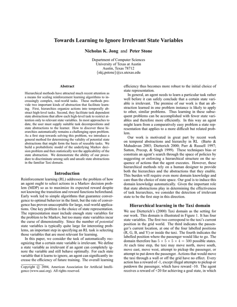
We use Dietterich’s (2000) Taxi domain as the setting for
our work. This domain is illustrated in Figure 1. It has four
state variables. The first two correspond to the taxi’s current
position in the grid world. The third indicates the passenger’s current location, at one of the four labelled positions
(R, G, B, and Y) or inside the taxi. The fourth indicates the
labelled position where the passenger would like to go. The
domain therefore has 5 × 5 × 5 × 4 = 500 possible states.
At each time step, the taxi may move north, move south,
move east, move west, attempt to pickup the passenger, or
attempt to put down the passenger. Actions that would move
the taxi through a wall or off the grid have no effect. Every
action has a reward of -1, except illegal attempts to pickup or
putdown the passenger, which have reward -10. The agent
receives a reward of +20 for achieving a goal state, in which
the passenger is at the destination (and not inside the taxi). In
this paper, we consider the stochastic version of the domain.
Whenever the taxi attempts to move, the resulting motion
occurs in a random perpendicular direction with probability
0.2. Furthermore, once the taxi picks up the passenger and
begins to move, the destination changes with probability 0.3.
stricted situations. In particular, we develop a procedure for
determining automatically that a state variable is irrelevant
conditional on the values of the other state variables. State
abstractions can be useful on their own in that they reduce
the number of parameters to be learned in the Q and value
functions. We leave for future work how one might generalize these conditions into temporal abstractions.
Defining irrelevance
Suppose without loss of generality that the n + 1 state vari~ and Y . Let X deables of an MDP are X1 , X2 , . . . Xn = X
~
note a set of possible values for X, determining a region of
the state space. We wish to determine whether or not knowing the value of Y affects the quality of an agent’s decisions
in this region of the state space. One simple sufficient condition is that the agent’s learned policy π̂ ignores Y :
∀~x ∈ X , y1 , y2 : π̂(~x, y1 ) = π̂(~x, y2 ).
Figure 1: The Taxi domain.
Dietterich demonstrates that a hand crafted task hierarchy,
shown in Figure 2, can facilitate learning in this domain. In
his MAXQ framework, each box corresponds to a subtask
hTi , Ai , R̃i i, where Ti is the set of states in which the subtask terminates, Ai is the set of permissible actions (denoted
by arrows in the figure), and R̃i is a function determining the
local reward the controller for that subtask earns for achieving each terminal state. This hierarchy reduces the problem
of learning a policy for the original domain into the problem of learning policies for each subtask. Note that once
an agent learns to navigate to each of the four landmark locations, it can apply this knowledge both when going to a
location to pickup the passenger and when going to a location to putdown the passenger. Without this abstraction, the
agent must waste time learning to navigate to each landmark
twice. Dietterich’s hierarchical learning algorithm also benefits from the knowledge that once you’ve decided to navigate to a certain position, the only relevant state variables
are the taxi’s coordinates.
Figure 2: A task decomposition for the Taxi domain.
How might a learning algorithm reach the same conclusion autonomously, based only on experience with the domain? Dietterich develops his framework by starting with
the temporal abstractions (the tasks) and then demonstrating
the state abstractions that apply within each task. In contrast,
we begin by recognizing state abstractions that apply in re-
However, this condition is too strong in practice. If some
states have more than one optimal action, then the learned
policy may specify one action when Y = y1 and a different
one when Y = y2 , due to noise in the learned Q values.
For example, the following table shows an optimal policy
for the stochastic taxi domain for the case when the passenger is in the upper left corner (and not yet in the taxi) and
wants to go to the lower right destination, obtained using Qlearning with Boltzmann exploration.1 Each cell in the table
displays the action for the corresponding position in the domain.
4 PickUp West
South South South
3
North
West
South South South
2
North
West
West
West
West
1 North
North North North West
0 North
North West
North North
0
1
2
3
4
The same Q-learning run produces the following similar policy for the case when the passenger instead wants to go to the
upper right destination.
4
3
2
1
0
PickUp
North
North
North
North
0
West
North
North
North
North
1
South
South
West
West
West
2
West
West
West
North
North
3
West
West
West
West
North
4
Since the passenger’s destination is irrelevant for the task of
first picking up the passenger, both of these policies are actually optimal for both passenger destinations. However, the
learned policies alone don’t support this conclusion. They
do not contain enough information to determine whether
they differ due to some actual significance of the passenger
destination or due to mere noise in the data.
We instead examine the state-action values themselves.
We check that in every case there exists some action that
1
For all the Q-learning runs in this paper, we used a starting
temperature of 50, a cooling rate of 0.9879, a learning rate of 0.25,
and no discount factor.
achieves the maximum expected reward regardless of the
value of Y :
∀~x ∈ X ∃a ∀y : Q̂(~x, y, a) ≈ V̂ (~x, y).
Our determination of whether an action maximizes the expected reward must be robust to noise in our value estimates.
Even if our learning algorithm converges to an optimal policy, we have no guarantee that it correctly estimates the value
of every optimal action. For example, for the Q-learning run
discussed earlier, consider the agent’s choice of action when
the taxi is in the upper right most square and the passenger is
at the Red landmark (in the upper left square). The agent’s
estimated values for each action are shown in Figure 3 for
two different passenger destinations. We can see at a glance
that the learned policy, indicated with solid arrows, is sensitive to a state variable we know to be irrelevant. If the passenger wants to go to the Blue (lower right hand) landmark,
the agent attempts to move west instead of south, since in
this particular run its learned value for attempting to move
south is only -9.42 and its learned value for attempting to
move west is -5.13. In contrast, if the passenger wants to go
to the Yellow (lower left hand) landmark, the agent attempts
to move south instead of west, for which the value estimates
are -0.55 and -6.83, respectively. In actuality, both attempting to move south and attempting to move west are optimal,
regardless of the passenger’s destination. For a given destination, the values of the two state-actions should be the
same, but the greedy aspect of the exploration policy causes
Q-learning to converge to an accurate estimate for only one
optimal action. The perceived difference in value between
equally good actions becomes less dramatic with more balanced exploration, but in general the stochasticity in the domain will always lead to some discrepancy. Our goal is to
define some criterion for determining when this discrepancy
is small enough to consider two actions equally good.
V=−1.89
V=−5.13
V=1.36
Q=−5.13
Q=−1.89
Q=−9.42
V=0.98
(a)
Q=−2.39
V=−2.39
V=−0.55
Q=−6.83
Q=1.36
Q=−0.55
V=2.94
Q=1.75
V=1.75
(b)
Figure 3: Estimated state values from Q-learning for a small
portion of the state space: the four upper right hand squares
in the domain. The passenger is at the Red landmark (not
shown). In (a), the passenger’s destination is the Blue landmark; in (b), the passenger’s destination is the Green landmark. For the upper right most square, the two optimal actions and their estimated values are shown. The learned policy is indicated with the solid arrows.
We adopt an approach inspired by statistical hypothesis
testing. For a given state (~x, y) and action a, we define our
null hypothesis as Q(~x, y, a) = V (~x, y), in which case a
is an optimal action in state (~x, y). If we accept the null
hypothesis for all y, then action a is optimal regardless of
the value of Y . According to our definition of irrelevance,
Y is irrelevant given ~x if any action is optimal regardless of
the value of Y . Conversely, Y is relevant given ~x if for every
action we reject the null hypothesis for some value of Y .
A straightforward implementation of this approach would
involve generating independent estimates of the underlying
MDP and then comparing the resulting Q values with a statistical test such as the Wilcoxon signed ranks test. This implementation would make very poor use of experience data,
since each time step would contribute to only one of the sample MDPs. Instead we draw upon recent work in Bayesian
MDP models. All of the data contributes to the Bayesian
model, from which we draw sample MDPs that are independent given the model. These samples allow us to make
probabilistic statements about the Q-values of the underlying MDP. We then accept an action as optimal unless the
probability of optimality is too low:
Q̂(~x, y, a) ≈ V̂ (~x, y) ≡
Pr(Q(~x, y, a) = V (~x, y) | h) ≥ p,
where h is the sequence of observed states, actions, rewards,
and successor states that led to our estimates Q̂ and V̂ .
Bayesian estimation for RL
Traditional model-based reinforcement learning algorithms
maintain a single estimate of the unknown parameters of
an MDP: the transition probabilities and one step reward
function. Dearden, Friedman, and Andre (1999) advocate
a Bayesian approach that maintains a full probability distribution over possible values for each parameter.
Consider the successor state s0 that results from executing
action a at state s. We can consider s0 a random variable
distributed according to a multinomial distribution with unt
known parameters θs,a
(a vector of probabilities for each
possible outcome) determined by the MDP’s unknown transition function. The task of learning an MDP’s dynamics
thus reduces to estimating the parameters of one multinomial distribution for each state-action pair s, a.
t
In the Bayesian approach to estimating θs,a
, we maintain
t
a probability distribution over possible values for θs,a
and
update this distribution every time we obtain a new sample from it. From the statistics literature, we know that the
multinomial distribution has a conjugate prior: the Dirichlet distribution. This means that if we assume a priori that
t
θs,a
is distributed according to a Dirichlet distribution with
certain parameters, then after conditioning on all the evidence the posterior distribution will also be Dirichlet, with
updated parameters. The parameters of a Dirichlet distribution are observation counts ui for each possible outcome si .
To each transition
function it assigns a probability proporQn
tional to i=1 pui i −1 , where pi (which must be positive) is
the probability of outcome i and n is the number
Pnof possible
outcomes. It can be shown that E[pi ] = ui / i=1 ui . The
update to the Dirichlet distribution after observing a certain
outcome i is simply an increment of ui .
In practice, this means that we can efficiently maintain
probability distributions over the unknown transition functions of the MDP. If we also have probability distributions
over the reward functions, then the joint distribution over
all these parameters defines a single probability distribution
over MDPs. This probability distribution only assigns a significant probability density to those MDPs that could have
plausibly generated the data. As more and more evidence
accumulates, fewer and fewer MDPs appear likely, and the
variance of the distribution decreases.
Although the mean of this probability distribution converges in the limit to the true underlying MDP, for small
amounts of data the accuracy depends on the choice of prior
distribution. In the work reported here, we used an improper
prior, in which we initialized each observation count to 0.
This prior is improper because the Dirichlet distribution is
formally defined only for ui > 0. However, observing that
limui →0 pi = 0 if the other ui remain fixed, we can interpret an improper Dirichlet distribution as a proper Dirichlet
distribution over the subset of outcomes with positive observation counts. This approach has the advantage that the
mean of our distribution over MDPs will be the same as the
maximum likelihood estimate of the MDP from the data.
Every other choice of prior from the Dirichlet distribution
necessarily introduces bias into the estimate of the underlying MDP.
Given a probability distribution over MDPs, we can make
probabilistic statements about arbitrary properties of an
MDP using a Monte Carlo approach. In particular, suppose
we want to estimate the probability that Q(s, a) = V (s).
We sample a suitably large number of MDPs from our distribution over MDPs and then observe how many times the
property holds. From this data, we can estimate the desired
probability directly.
Note that the a priori probability that any given action is
optimal at a given state is inversely proportional to the number of actions. As the distribution over MDPs approximates
the true MDP increasingly well, this probability of optimality will converge to 0 for all suboptimal actions. All the
probability mass will converge to the set of optimal actions,
though the distribution among these actions will depend on
noise in the samples from the true MDP.
Results
Discovering state abstractions
To test the validity of our approach, we applied our state
abstraction discovery method to the stochastic version of the
Taxi domain. We used prioritized sweeping (Moore & Atkeson 1993) with tBored = 10 to ensure that the Bayesian
model had at least ten samples for each reachable transition function.2 We allowed the agent to explore for 50,000
time steps, enough to ensure that the it completed its exploration. The agent assumed that the reward function was deterministic, so it knew all the one step rewards after visiting
each state-action pair at least once. In general, if we do not
2
The other parameters we used for the prioritized sweeping algorithm were β = 5 sweeps per step and a minimum priority of
= 0.001 before placing a state in the priority queue.
make this assumption, then we must choose some prior distribution over rewards for each state-action pair. Since the
Taxi domain has a deterministic reward function, we chose
to avoid this complication in the work reported here. In principle, introducing variance into our estimates for the reward
function will reduce the certainty in the learned values somewhat, requiring some more exploration to compensate.3
After the exploration phase, we sampled 100 MDPs from
the learned Bayesian model. We examined situations in
which the taxi is navigating to the passenger’s source location. The optimal policy in these states may ignore the passenger’s destination location. For each possible value of the
taxi position and the passenger’s source, we estimated the
probabilities that each action was optimal across the three
possible values of the passenger’s destination. According
to our definition for irrelevance, we may conclude that the
passenger destination is irrelevant if some action is optimal
with probability at least p for all three destinations. Consider for example choosing p = 0.05. If the probability
that an action is optimal is smaller than 0.05, then we consider that action suboptimal. If every action is suboptimal
for some value of a given state variable, then we do not conclude that the state variable is irrelevant. Hence the smaller
the value of p, the more aggressively we classify actions as
optimal and thus state variables as irrelevant. The table below summarizes a typical result of this test for each taxi position, given that the passenger source is the Red (upper left
hand) square. Each probability shown is the largest value of
p that would allow us to conclude that the destination is irrelevant. That is, each cell represents for a given ~x the quantity
maxa miny P̂r(Q(~x, y, a) = V (~x, y)).
4
3
2
1
0
1.00
1.00
0.99
1.00
1.00
0
1.00
0.66
0.81
1.00
1.00
1
1.00
1.00
1.00
0.34
0.28
2
0.20
0.21
1.00
1.00
0.99
3
0.77
0.47
1.00
0.67
0.56
4
Note that the p-value is 1 or 0.99 in squares where only
one direction leads optimally to row 4, column 0; any choice
of p would allow us to conclude that passenger destination is
irrelevant at these positions. The intermediate values correspond to positions in which the taxi has two optimal actions.
Since the smallest of these is 0.20, any choice of p ≤ 0.20
would allow us to conclude that passenger destination is irrelevant in this case.
The next table shows the result of the test for the case
when the passenger is in the taxi. In this case, the passenger’s destination generally is relevant to the agent’s ability
to behave optimally. As the p-values suggest, there are four
positions where one action is optimal across all four passenger destinations: moving north, to get around the two vertical walls at the bottom of the grid. In every other cell, no
one action is optimal across all four passenger destinations.
3
Dearden, Friedman, and Andre (Dearden, Friedman, & Andre
1999) model rewards as multinomial distributions the same way
they model transition functions, but as a result they must supply a
priori some finite set that contains all possible rewards.
(Recall the possible passenger destinations as indicated in
Figure 1.)
0.00
0.00
0.00
0.00
0.00
0
0.00
0.00
0.00
0.23
0.79
1
0.00
0.00
0.00
0.74
0.64
2
0.00
0.00
0.00
0.00
0.00
3
0.00
0.00
0.00
0.00
0.00
4
The numbers in these two tables indicate that the agent is
able to determine automatically that the passenger’s destination is only relevant once the passenger has been picked up.
Thus while the passenger is still at its source location, the
agent can learn with a smaller state representation, allowing
it to learn more efficiently.
The results shown above are typical, though as with all
forms of statistical hypothesis testing, the above procedure
will occasionally yield a very low probability that an action is optimal even though the action actually is optimal.
We can reduce the chances of such an error by choosing a
suitably small value for p, although extreme values require
larger samples to test accurately.
Applying state abstractions
We have demonstrated a method that can detect irrelevant
state variables, but only after already solving the task. The
state abstractions learned from solving a task do not confer
any further benefit for that task, but they do allow learning
algorithms to learn related tasks more efficiently, simply by
aliasing together the appropriate states. For example, suppose that after an agent masters the Taxi domain, we present
it with another domain that differs only in the location of the
four landmarks. (We allow the agent to know that the task
has changed somewhat.)
Since the effects and one step rewards for executing the
pickup and putdown actions have changed, our prioritized
sweeping agent cannot directly reuse the model learned from
the first task. In contrast, the learned state abstraction continues to apply. As seen in Figure 4, the state abstraction
enables prioritized sweeping to learn the revised task twice
as quickly.
Since the abstraction reduces the size of the state space
from 500 to 300, it is not particularly surprising that prioritized sweeping learns more quickly, given that it explicitly tries each action a certain number of times from each
reachable state (tBored times). However, the learned state
abstraction in the Taxi domain also benefits learning algorithms that do not explicitly take time proportional to the
state size. Figure 5 shows the results of reproducing the
above experiment with the Q-learning algorithm. Again, the
ability to transfer domain knowledge in the form of a state
abstraction speeds learning by a factor of 2. Also, we see
that a naive attempt to transfer domain knowledge in the
form of Q values worsens performance relative to starting
from scratch, since the agent must first unlearn the old policy.
The primary cost of applying this technique is computational. Sampling and then solving 100 MDPs from the
Bayesian model of the Taxi domain required almost eight
With abstraction
Without abstraction
0
Average reward per episode
4
3
2
1
0
Prioritized Sweeping in a Random Taxi Domain
1000
-1000
-2000
-3000
-4000
-5000
-6000
0
5000
10000
15000
20000
25000
Number of primitive actions
30000
35000
40000
Figure 4: Average reward per episode on a new task, with
and without the state abstractions learned from the first task.
Each curve is the average of 25 runs.
minutes of CPU time on a 2.4GHz Intel Pentium 4 processor, though we have not yet performed any optimizations
such as tuning the number of samples required. Solving a
random Taxi domain directly, without any learned state abstraction, took less than a second with Q-learning and less
than thirty seconds with prioritized sweeping. Searching for
state abstractions in this manner hence seems most beneficial when the cost of taking an action in the environment is
relatively high and the cost of computation time is relatively
low. Alternatively, we imagine applying this technique to
find state abstractions in small examples that might apply to
much larger problems of real interest. However, such applications would likely require a method for verifying that a
state abstraction learned in one task applies to a new task.
The procedure described in this paper also leaves open
the questions of when and how to determine what abstractions to test. We allowed the agent to explore the environment sufficiently before testing for state abstractions, but we
don’t yet have a general method for determining how much
exploration is sufficient. If the model of the environment is
too uncertain, the procedure will conclude that most actions
could be optimal and thus aggressively abstract away actually relevant state variables. We also leave for future work
the details of how to choose what state variables to test for
irrelevancy and how to determine precisely under what conditions these local state abstractions apply.
Related work
Other researchers have addressed the problem of finding
state abstractions for hierarchical RL. The most closely related work to ours is Jonsson and Barto’s (2001) usage of
U-trees to discover state abstractions for options. They assume that the hierarchy (in the form of the options) is given,
and then apply U-trees to learn the state representation and
policies for each task. However, this approach relies on the
given options to provide local contexts in which the abstractions apply uniformly. In contrast, our approach develops a
Q-Learning in a Random Taxi Domain
100
With abstraction
Without abstraction
Initialized with old Q values
Average reward per episode
0
-100
-200
-300
-400
-500
-600
0
5000
10000
15000
20000
25000
Number of primitive actions
30000
35000
40000
Figure 5: Average reward per episode on a new task, with
state abstraction, without state abstraction, and without state
abstraction but with Q values remembered from the first
task. Each curve is the average of 25 runs.
general test for relevancy that we hope will lead eventually
to the discovery of these contexts themselves.
Hengst (2002) discovers both a hierarchy and state abstractions for the Taxi domain using a variable-ordering
heuristic. He observes that the taxi location changes much
more frequently than the passenger location, which itself
changes more frequently than the passenger’s destination.
His approach constructs a hierarchy with one level for each
variable, identifying what actions allow the agent to transition among levels. Again, our goal is to develop a general
method for discovering abstractions and then hierarchies in
arbitrary environments, including those where the variables’
frequency of changing values doesn’t provide enough information.
Conclusion
This paper introduces a Bayesian approach to determining the relevance of a state variable for behaving optimally
within an arbitrary region of the state space. Our empirical
results in a representative task instance demonstrates that the
procedure can discover state abstractions accurately and that
these state abstractions significantly improve the learning of
similar tasks. We believe that this technique will provide the
foundation for a principled mechanism for the automatic discovery of dynamic state abstractions, which in turn may give
rise to the automatic discovery of useful task hierarchies.
References
Barto, A. G., and Mahadevan, S. 2003. Recent advances
in hierarchical reinforcement learning. Discrete-Event Systems 13:41–77. Special Issue on Reinforcement Learning.
Dearden, R.; Friedman, N.; and Andre, D. 1999. Model
based Bayesian exploration. In Proceedings of the Fifteenth Conference on Uncertainty in Artificial Intelligence,
150–159.
Dietterich, T. G. 2000. Hierarchical reinforcement learning
with the MAXQ value function decomposition. Journal of
Artificial Intelligence Research 13:227–303.
Hengst, B. 2002. Discovering hierarchy in reinforcement
learning with HEXQ. In Proceedings of the Nineteenth
International Conference on Machine Learning.
Jonsson, A., and Barto, A. G. 2001. Automated state abstraction for options using the U-tree algorithm. In Advances in Neural Information Processing Systems 14.
Moore, A. W., and Atkeson, C. G. 1993. Prioritized sweeping: Reinforcement learning with less data and less real
time. Machine Learning 13:103–130.
Parr, R., and Russell, S. 1997. Reinforcement learning
with hierarchies of machines. In Advances in Neural Information Processing Systems 10.
Sutton, R. S.; Precup, D.; and Singh, S. 1999. Between
MDPs and semi-MDPs: A framework for temporal abstraction in reinforcement learning. Artificial Intelligence
112(1–2):181–211.