State Estimation for Game AI Using Particle Filters
Curt Bererton
curt@cs.cmu.edu
Carnegie Mellon University
5000 Forbes Ave
Pittsburgh, PA 15217
Abstract
Artificial intelligence for games is a challenging area in that
it has tight processing constraints and must be fun to play
against or with. Some of the latest techniques from robotics
research are likely to be applicable to game AI. In particular,
we propose that particle filters are well suited to the game AI
problem. In this paper, we introduce particle filters, justify
their use in game AI, and show the results implemented in a
simple game developed using the crystal space game engine.
Introduction
gent, it doesn’t matter what AI (if any) was actually implemented to achieve that illusion”(Liden 2003).
On the surface, this seems to be a reasonable statement.
We argue that this statement may lead AI developers down
a path with an unsatisfactory result. The base question is:
Is it easier to give the illusion of intelligence, or to make
something actually be intelligent?
The problem with AI in today’s games is that they do not
give us the illusion that the NPC is very intelligent, although
there have been some excellent efforts in this direction. We
argue that the best way to give NPCs the illusion of intelligence is to actually give them intelligence using a computationally efficient method.
It is clear that, in most any game, NPCs are using too
much omniscience against us. Thus the question becomes,
what omniscient information should we use to make the AI
smarter and what omniscient information should we conceal
from the agent to make the AI dumber.
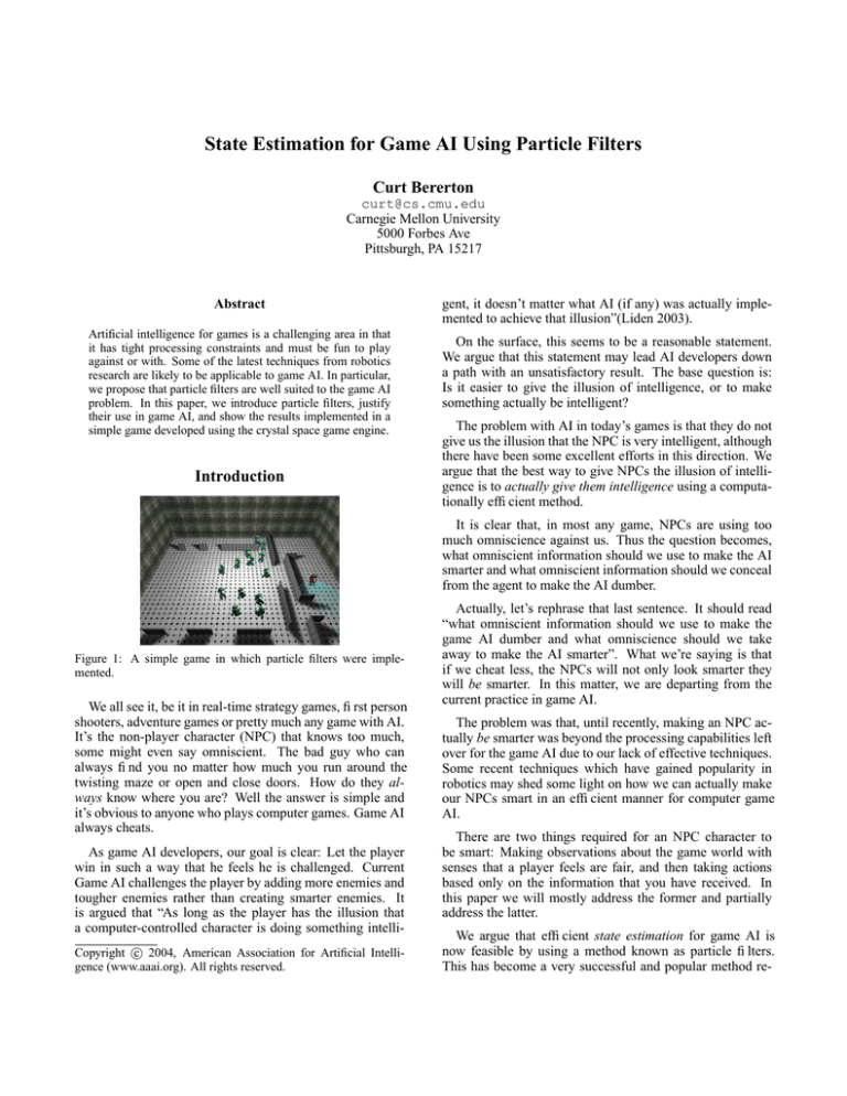
Figure 1: A simple game in which particle filters were implemented.
We all see it, be it in real-time strategy games, first person
shooters, adventure games or pretty much any game with AI.
It’s the non-player character (NPC) that knows too much,
some might even say omniscient. The bad guy who can
always find you no matter how much you run around the
twisting maze or open and close doors. How do they always know where you are? Well the answer is simple and
it’s obvious to anyone who plays computer games. Game AI
always cheats.
As game AI developers, our goal is clear: Let the player
win in such a way that he feels he is challenged. Current
Game AI challenges the player by adding more enemies and
tougher enemies rather than creating smarter enemies. It
is argued that “As long as the player has the illusion that
a computer-controlled character is doing something intellic 2004, American Association for Artificial IntelliCopyright gence (www.aaai.org). All rights reserved.
Actually, let’s rephrase that last sentence. It should read
“what omniscient information should we use to make the
game AI dumber and what omniscience should we take
away to make the AI smarter”. What we’re saying is that
if we cheat less, the NPCs will not only look smarter they
will be smarter. In this matter, we are departing from the
current practice in game AI.
The problem was that, until recently, making an NPC actually be smarter was beyond the processing capabilities left
over for the game AI due to our lack of effective techniques.
Some recent techniques which have gained popularity in
robotics may shed some light on how we can actually make
our NPCs smart in an efficient manner for computer game
AI.
There are two things required for an NPC character to
be smart: Making observations about the game world with
senses that a player feels are fair, and then taking actions
based only on the information that you have received. In
this paper we will mostly address the former and partially
address the latter.
We argue that efficient state estimation for game AI is
now feasible by using a method known as particle filters.
This has become a very successful and popular method re-
cently in the field of robotics in a variety of applications including robot soccer (Thrun 2002).
Robotics has many of the same limitations as game AI.
Decisions must be made quickly to react with environments
changing in real-time. The processor is spending much of
its time processing observations, running motors, and other
functionality unrelated to AI and not much is left for thinking. Thus, we argue that methods successful in robotics are
likely to also be successful in game AI.
In particular, we hope to convince the reader that particle
filters are such a method. They have the ability provide information to the AI about the state of the world in much the
same way as a person would receive information about the
state of a world. They can also do so in a computationally
efficient manner. They are tunable; Given more computing
time they are “smarter”, given less time they are “dumber”.
This can be used by the game designer to tune the intelligence of NPCs in the game so that instead of having to make
enemies more abundant or tougher, we can finally just make
them actually smarter and thus more of a challenge.
First, we will describe the typical scenario where it’s obvious to the player that the AI is cheating and describe the
problem that we will address with this work. We will present
some background on state estimation and the basic mathematics of particle filters. Then we will show how these
methods can be applied to game AI. The results of this application are shown in a simple game created using the crystal space game engine. A screenshot of our game is shown
in figure 1. We will then conclude with the future directions
this technology may lead.
We know you’re cheating: The problem with
too much omniscience
PLAYER
ROOM #1
NPC
ROOM #2
ROOM #3
Figure 2: How does the NPC always know to go straight to room 2
where the player chose to hide instead of checking room 1 first?
It’s obvious to anyone who has ever played against any
game AI that the NPCs always know where you are. Take,
for example, figure 2 above. The player runs away from an
NPC who is down the hall and begins to chase. The player
hides in room two. The NPC never stops to check room one
or ever passes past room two, it will always go directly to the
player (although we might make it take more or less time).
Why does the NPC do this? Well the NPC is cheating. It
always knows where the player is. It is too omniscient.
Even more so, it doesn’t even have the capability to reason
about where the player might be, so that it cannot possibly
make decisions based on looking where the player might be
or guessing one of the possible locations of the player. We
argue that determining information about where the player
might be in a reasonable manner will open a brand new set
of options to the game AI programmer and to the game designer. One could actually search for the player, or coordinate groups of agents to perform this search.
In the example above, let us overlay the map with a coarse
grid of cells, perhaps the same set of coarse grid cells being
used for path planning such as those proposed for game AI
path planning in (Dickheiser 2003; van der Sterren 2003).
If we give each grid cell a boolean variable with values
“player not here” or “player possibly here”, then we can use
this information to reason about where a player might be.
With this information we can have the NPC search the map
room by room for the player, or randomly choose rooms to
check. When the NPC looks somewhere and doesn’t see the
player, we can mark all of the grid cells in that area with
“player not here” and then look elsewhere. Knowing where
the player is or might be is a form of state estimation. We
will talk more about state estimation in the next section
All we need is a way to update our grid of boolean variables so that it correctly represents where the player might
be, given what all or some group of the NPCs on the map can
see. There are mathematically sound, and computationally
efficient methods to perform the task of state estimation. In
this paper, we will concentrate on using particle filters.
Background
Firstly, let us define what we mean by state. The “state” of
a system is typically a vector of variables which contains
all the relevant information required to describe the system
under investigation. We will use the notation x to denote the
state vector and xt to denote the state of the system at time
t. When a system is fully observable, then the entire state
vector x is known. Typically, the next state of the system is
a function f () (possibly non-linear) of the previous state and
some noise vt : xt+1 = f (xt , vt ). In this paper, the state we
are typically interested in will be the position of the player.
Thus the state vector xt will consist of the position of the
player, or possibly the position of all players in the game.
In robotics, it is often impossible to observe state variables (such as the position of your robot, or other robots in
the area) directly. They are often measured using observations which are a noisy function of the state. We will denote
observations using z where an observation is a noisy (with
noise n) function of the state: zt = h(xt , nt ). A typical
observation might be “I cannot see the player in a particular
viewing radius, or “I can see the player and she is at position
(x,y)”.
In a typical computer game, the state of interest to an AI
agent is the location, orientation, velocity and possibly other
information about a given player, set of players, or other automated agents in the game. With partial or full knowledge
of this information, the bot or AI agent can reason about
what actions should be performed to either attack or assist
the players or other agents.
NPC
PLAYER
The problem in game AI is that we always use the entire
state of the player including their position, orientation, velocity etc. to find the player. Why would we spend effort
reasoning about what an NPC might believe about the state?
The answer is simple: If you do not reason about observing
the state of the other agents in the game and simply use the
full known state to perform behaviors or run state machines,
then your agent will be cheating and it will be obvious to
anyone who sees it act in the game. In fact, what we’d like to
do is calculate a belief state: A probability distribution that
the NPC maintains which reflects what the NPC or NPCs
know about the true state of the player. This is done by incorporating realistic observations that the NPC could have
made using vision or hearing.
Particle Filters for Game AI
Assume that we have a prior probability distribution over
the location of single player in the map. That is we have
some guess in the form of a probability distribution p over
the state at time 0 as p(x0 ). This corresponds to how likely it
is for the player to be at a given location. ie. we might start
assuming the player is equally likely to be at any location,
or we might say that the player starts at an exact point on the
map.
We will reason about the state of the player xt in discrete
time steps. This is typically valid in computer games, since
calculations are performed at each frame to be rendered. The
method still applies if the interval between time steps varies.
What we would like to determine is a posterior probability
distribution over where the player might be given the observations of one or more NPCs on the same map. This posterior probability distribution over the state is also known as
the belief state. That is we are trying to determine where
we think the player might be at time t given our initial guess
p(x0 ) and all the observations of the state at every time step
until the present time: z0..t .
A solution to this problem is provided by Bayes filters
(Jazwinsky 1970). Bayes filters give us a recursive solution
to estimating the probability of the player being in any location at the current time xt given the observations zt . That is,
given a guess at the initial state, we recursively estimate the
position of the player at time t by incorporating measurements at each time step. The general equation for a Bayes
filter is shown in equation (1).
p(xt |zt ) = c · p(zt |xt )
Z
xt−1
p(xt |xt−1 )p(xt−1 |zt−1 )dxt−1
(1)
Equation (1) can be worded in English as follows: the
probability that the state is x at time t given the most recent
PLAYER
NPC
Figure 3: Left: Particles (the small shaded circles) represent possible locations of the player. Right: As the NPC searches, particles in
the NPC’s line of sight when the player is not present are removed
measurement is equal to the probability of the current measurement zt given that the robot might be in state x times the
likelihood of being in state x given our belief and measurements at the previous time steps multiplied by a normalizing
constant c.
A Bayes filter is equivalent to the well known Kalman
filter (Kalman 1960) if we use gaussian distributions to represent the probability distributions above. Although Kalman
filters are efficient state estimators, they are most useful for
distributions with single modes and next states which are a
linear function of the prior state and known gaussian noise.
Kalman filters are not well suited to game AI because we
cannot reason about situations such as “the player is either
in room one, room two or room 3”, since that scenario would
not be well represented by a gaussian distribution.
Particle filters represent the probability distributions in
equation (1) using a non-parametric representation. That is,
it will represent the distribution as a set of weighted samples
(known as particles) from that distribution. Each sample xi
has a weight wi , where i is an integer index for a given sample. Typically, we will represent a probability distribution
using a fixed number of samples Ns . The wi sum to one:
P
i wi = 1.0.
The algorithm
We have implemented one of the simplest versions of the
particle filter to demonstrate its use in a computer game.
There are an almost infinite number of particle filter variations, but we have chosen to implement the Sampling Importance Resampling Filter version of the particle filter described in (Arulampapam et al. 2001). The algorithm
(shown in figure 4) is trivial to implement and requires only
a couple pages of code in C++.
This algorithm is called repeatedly at each time step or
frame. A more intuitive description of the algorithm in our
game world follows. Each sample corresponds to a possible
location of the player. The sample data structure has an x and
y position and a weight associated with it. Particle filtering
consists of three main steps. The first step, generating a proposal distribution, asks “Where could the player have moved
to now given what I knew about where he might have been
an instant before. The second step, incorporating observations, asks “given what I can see, update my belief about
Ns
i
i
s
[{xit , wti }N
i=1 ] = SIR[{xt−1 , wt−1 }i=1 , zt ]
Generate proposal distribution:
for i = 1 : Ns
Draw a sample xit from p(xt |xit−1 )
end for
Incorporate observations:
for i = 1 : Ns
Calculate wti = p(zt |xit )
end for
Renormalize the weights to sum to one:
PN s
t = i=1
(wti )
for i = 1 : Ns
wi
wti = tt
end for
Resample the distribution according to
(Arulampapam et al. 2001):
i
i Ns
s
[{xit , wti }N
i=1 ] = RESAM P LE[{xt , wt }i=1 ]
Figure 4: The Sampling Importance Resampling particle filter.
where the player is”. The third, resampling, is required for
the filter maintain diversity.
When generating a proposal distribution we used:
p(xt |xit−1 ) to be brownian motion. That is, we took a given
input particle and added a random number to the x and y coordinate. This essentially means that the player may move
randomly or purposefully, but still be found.
By incorporating observations, we are referring to incorporating observations from the NPC characters in the map.
Our observation model consists of two modes. If the player
is visible by the NPC, then all particles are weighted proportional to their distance from the player. If the player is
not visible by the NPC, then we use a replication of a laser
range finder to mimic the field of view of an NPC agent.
Thus we send out a set of rays from the NPC as depicted in
figure 5. Particles that are close to the ray have a low probability, since the NPC can see there, and the player is not
visible. This has the effect of removing the particles where
the player can see, thus the NPC can sweep the environment
of particles. Any location where there are particles remaining is a possible location of the player. Areas containing
particles indicate an area where the player may reside.
The resampling procedure simply resamples particles according to the renormalized weights. Particles with higher
weights get sampled more often than particles with lower
weights.
Computationally, the above algorithm is linear in the
number of samples multiplied by the number of laser range
finder lines used in the observation model O(Ns · Nlasers ).
The beauty of particle filters is that they can be tuned to let
an agent be “smarter” or “dumber” simply by changing the
number of particles used. Thus, particle filtering is consid-
ered to be an “anytime” algorithm. We can stop processing
whenever we run out of time. If we have more time, we’ll
get a more accurate answer. If we have less time, the answer
will not be as precise because we are using less particles to
represent the posterior probability distribution.
NPC
PLAYER
Figure 5: This figure depicts the laser range finding lines that form
the NPC observation model.
Results on a simple game
The game consists of two teams of robots on a two dimensional map. One team is controlled either by a human or
an NPC and the other team is always controlled by NPCs.
The objective is simply to defeat the other team by throwing blocks at the other team. It takes four hits to disable a
robot, and you can only have one block in the air at a time.
A screenshot of the game is shown in figure 1.
We find that, on the maps we use, between 200 and 500
particles are sufficient in order to represent the possible locations of the player. Larger maps require more particles.
We use about 10 laser range finder measurements per NPC
when there are fewer NPCs on the map, and only about two
or 3 measurements when there are many NPCs on screen.
For every laser range finder measurement we perform one
line of sight test to the nearest obstacle on the map, one distance calculation and possibly one cross product per particle. These computations require a minimum percentage of
the CPU processing power.
A simple controller for the NPCs is used. The NPC tries to
navigate to the mean of the posterior distribution (the middle
of the cloud of particles). This had the desirable effect of
clearing particles from one area and then causing the NPC
to search a new area.
We ran experiments with up to thirty agents searching for
a single player at which point computation was such that
it started to slow the frame rate of the game to below 25
frames per second. During this final experiment, the player
also tracks each of the NPCs using a particle filter. In total,
there are 31 particle filters being executed simultaneously
tracking 31 agents. The experiments were performed on a
1.0 GHz pentium 4 with 500MB of memory running Red
Hat 9.0. None of the code was optimized to any extent either
by the compiler or the programmer.
In another experiment, we reduced the number of particles
to see what occurs when there were not enough to cover the
map. The NPCs still search the map, but it is often the case
that they believe the player to be in an area in which they
are not. Thus the NPCs search the area randomly. If they
ever cause the posterior probability to drop below a threshold, we restart the particle filter with the particles distributed
evenly over the map. In all, this particle starvation created
a reasonable random searching method by the agents. They
would randomly check various areas of the map. Thus, given
less computation particle filters with a simple controller still
yields reasonable behavior.
While a picture is worth a thousand words, clearly
a video would better be able to show the capabilities
of particle filtering. We have created a short video
of our game engine using particle filters. Please visit
www.cs.cmu.edu/∼curt/research.html for more information.
Suggested modifications and control methods
Changing the proposal distribution from a brownian motion
based model to something more similar to a pursuit evasion
style model such as in (Parsons 1976) using the navigation
grids already available (Dickheiser 2003; van der Sterren
2003), would greatly improve performance.
There are reasonable approximations to the optimal solution of finding an adversary under uncertainly only now
becoming available (Roy & Gordon 2002). There is also a
large body of literature on pursuit evasion which can also be
applied to this problem (Gerkey 2004).It is possible that the
above methods can be optimized sufficiently to be of use for
games. However, it is more likely that, in the near future,
particle filters will be used with another control method familiar to the game industry such as state machines, neural
nets, or hand coded behaviors.
One effective method would be to have the level designer
or an algorithm predefine a set of areas in the map. The NPC
controller could then look in the nearest area which hasn’t
been cleared of particles. Or agents could bid on rooms
which they wanted to search using auction methods which
have recently become popular in robot soccer and multirobot control (Vail & Veloso 2003; Zlot et al. 2002).
With any choice of controller, we can then have the NPCs
display their new found intelligence to the player by making
statements such as: “I’m going to check the living room”,
or “Bob! Check the barracks!”. Another interesting feature
would be to display the particles to the player after the fact
to show the player exactly how the AI beat them.
One could also allow for more or less coordination between the agents. For instance each NPC tracking the player
could have its own particle filter. A new type of observation might be information from a second NPC that they had
checked certain areas, at which point those areas would be
cleared. If the player were in earshot, this form of communication might come via radio that “Bob, I’ve checked
the living room and the barracks and I didn’t see anything”.
Particle filters also would allow misdirection. The player
throwing a rock into a distant room could be treated as an
observation which would cause the NPC to search that room.
Needless to say, this would allow for new types of game play
currently unavailable.
Conclusions and Future Directions
The objective of this paper is to introduce state estimation
to the field of game AI and justify its use. In particular,
we present particle filters as a theoretically sound and computationally efficient method by which NPCs can track the
location of a player or other agents in a map. Using this information can lead to a variety of new game play and agents
capable of reasoning about future actions based on realistic
estimations of the player’s position.
It is also the author’s view that techniques are now becoming available to actually give computer controlled characters
useful intelligence using computationally efficient methods.
Since actual intelligence is cheap to achieve, why give the
player the illusion of intelligence, when the real thing is possible within our limitations?
References
Arulampapam, S.; Maskell, S.; Gordon, N.; and Clapp,
T. 2001. A tutorial on particle filters for on-line nonlinear/non-gaussian bayesian tracking. Available at: citeseer.org.
Dickheiser, M. 2003. AI Game Programming Wisdom.
Charles River Media, 2nd edition. chapter 2.2 Inexpensive
Precomputed Pathfinding Using a Navigation Set Hierarchy, 103–113.
Gerkey, B. 2004. Clear the building: Pursuit-evasion with
teams of robots. Submitted to:Advances in Artificial Intelligence, AAAI.
Jazwinsky, A. 1970. Stochastic Processes and Filtering
Theory. Academic Press.
Kalman, R. E. 1960. A new approach to linear filtering and
prediction problems. Journal of Basic Engineering.
Liden, L. 2003. AI Game Programming Wisdom. Charles
River Media, 2nd edition. chapter 1.4 Artificial Stupidity:
The Art of Intentional Mistakes, 41–48.
Parsons, T. 1976. Pursuit-evasion in a graph. Lecture
Notes in Mathematics. Springer-Verlag. chapter Theory
and Applications of Graphs, 426–441.
Roy, N., and Gordon, G. 2002. Exponential family PCA for
belief compression in POMDPs. In Becker, S.; Thrun, S.;
and Obermayer, K., eds., Advances in Neural Information
Processing 15 (NIPS), 1043–1049.
Thrun, S. 2002. Particle filters in robotics. In Uncertainty
in Artificial Intelligence (UAI).
Vail, D., and Veloso, M. 2003. Dynamic multi-robot coordination. Multi-Robot Systems: From Swarms to Intelligent
Automata.
van der Sterren, W. 2003. AI Game Programming Wisdom.
Charles River Media, 2nd edition. chapter 2.3 Path LookUp Tables - Small Is Beautiful, 115–129.
Zlot, R.; Stentz, A.; Dias, M.; and Thayer, S. 2002. Multirobot exploration controlled by a market economy.