From: AAAI Technical Report WS-02-13. Compilation copyright © 2002, AAAI (www.aaai.org). All rights reserved.
Utility Functions for Ceteris Paribus Preferences
Michael McGeachie
Jon Doyle
Laboratory for Computer Science
Massachusetts Institute of Technology
Cambridge, MA 02139
mmcgeach@mit.edu
Department of Computer Science
North Carolina State University
Raleigh, NC 27695-7535
Jon Doyle@ncsu.edu
Abstract
Although ceteris paribus preference statements concisely
represent one natural class of preferences over outcomes or
goals, many applications of such preferences require numeric
utility function representations to achieve computational efficiency. We provide algorithms, complete for finite universes
of binary features, for converting a set of qualitative ceteris
paribus preferences into quantitative utility functions.
Introduction
Although researchers have developed several logical representations of preference information (Doyle, Shoham, &
Wellman 1991; Mura & Shoham 1999; Bacchus & Grove
1996), development of adequate means for automated reasoning within and computational use of these representations remains an underexplored topic. To improve the utility
of these representations for practical applications, we consider the task of constructing or compiling numeric utility
functions to fit logical preference specifications, and present
algorithms for this task appropriate to the ceteris paribus
logic of Doyle, Shoham, and Wellman (1991).
Wellman and Doyle (1991) observed that ceteris paribus
preference provides a natural interpretation of a common
type of human preference, and built on this to develop
logical and mathematical formalizations of such information (Doyle, Shoham, & Wellman 1991; Doyle & Wellman
1994). Ceteris paribus preferences express preference comparisons over sets of possible worlds or outcomes characterized in terms of a set of binary features . Then each ceteris
paribus rule specifies some features of outcomes, and a preference over them, while ignoring the remaining features, the
intent being that comparisons hold the ignored features constant.
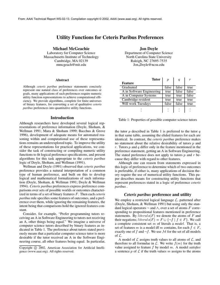
Consider, for example, “Prefer programming tutors receiving an A in Software Engineering to tutors not receiving
an A, other things being equal.” We imagine a universe of
computer science tutors described by binary features as indicated in Table 1. The preference about tutors stated previously means that a particular computer science tutor is more
desirable if the tutor received an A in the Software Engineering course, all other features being equal. In particular,
­
Copyright c 2002, American Association for Artificial Intelligence (www.aaai.org). All rights reserved.
Tutor
Feature
Graduated
A in Software Engineering
A in Computer Systems
Cambridge resident
Will work Tuesdays
..
.
false
true
true
true
false
..
.
false
false
true
true
false
..
.
true
false
false
true
true
..
.
Table 1: Properties of possible computer science tutors
the tutor described in Table 1 is preferred to the tutor in that same table, assuming the elided features for each are
identical. In contrast, the ceteris paribus preference makes
no statement about the relative desirability of tutors and
. Tutors and differ only in the feature mentioned in the
preference statement, getting an A in Software Engineering.
The stated preference does not apply to tutors and because they differ with regard to other features.
Although one can reason from statements expressed in
this logic of preference to determine which of two outcomes
is preferable, if either is, many applications of decision theory require the use of numerical utility functions. This paper describes means for constructing utility functions that
represent preferences stated in a logic of preference ceteris
paribus .
Ceteris paribus preference and utility
We employ a restricted logical language , patterned after
(Doyle, Shoham, & Wellman 1991) but using only the standard logical operators and , over a set of atoms corresponding to propositional features mentioned in preference
statements. By we denote the atoms of and
their negations; . We call
a complete consistent set of literals a model. That is, a
set of features is a model iff contains, for each ,
exactly one of and . We use for the set of all models
of .
A model of assigns truth values to all atoms of , and
therefore to all formulae in . We write for the truth
value assigned to feature by model . A model satisfies
a sentence of if the truth values assigns to the atoms
of make true. We write when satisfies . We
define the proposition expressed by a sentence , denoted by .
A preference order is a complete preorder (reflexive and
transitive relation) over . When , we say that
is weakly preferred to . If and , we
write and say that is strictly preferred to .
and , then we say is indifferent to
If , written . A utility function Ê maps
each model to a real number. A utility function represents
a preference order just in case whenever
.
We define a new language r of preference rules or preference constraints to consist of statements of the form, for
, of , meaning is desired at least as much as
, and , meaning is desired more than . Models of
r consist of preference orders over models of . We define
the meaning of preference rules in terms of the notions of
-model equivalence and modification.
is the minimal set of
The support of a sentence atoms determining the truth of , denoted . The support
of is the same as the set of atoms appearing in an irredundant sum-of-products sentence logically equivalent to .
Two models and are equivalent modulo if they are
the same outside the support of . Formally, iff
Model modification is defined as follows. A set of model
modifications of making true, written , are those
models satisfying which assign the same truth values to
atoms outside the support of as does. That is,
Formally, we say that a preference order satisfies if and only if for all in , and , we have . This means that when two
models assign the same truth values to all features not in
the support of either or , one making true and false
is weakly preferred to one making false and true. The
preference order satisfies a strict ceteris paribus preference
if and only if in addition some case has a model makes
true and false strictly preferred to one making false and
true.
For a preference rule , we write to denote the set of
preference orders over that satisfy , that is, consistent
with the constraint expressed by . We write for a set of
preference rules to denote the set of orders consistent with
. Consistent rules and
each , that is, rule sets admit at least one consistent preference order. If a
preference rule implies that , for ,
we write . For a set of preference rules, we
write to mean that for each .
We define the support of , denoted , to be the set
of features in present in the support of statements of appearing in constraints in . Formally, contains those
features such that either or appears in .
The following examines the problem of constructing, for
a finite set of ceteris paribus preference rules, a utility
function that represents some order in .
Intermediate representation
The utility construction methods developed here employ an
intermediate representation in terms of simple rules that relate paired patterns of specified and “don’t care” feature values.
Let be a finite set of preference rules. Because each
preference rule mentions only finitely many features, is also finite, and we write to mean .
We construct utility functions representing the constraints
in in terms of model features. Features not specified in
any rule in are not relevant to compute the utility of a
model, since there is no preference information about them
in the set . Accordingly, we focus our attention on .
We define the intermediate representation relative to an
enumeration of .
We define the language r of intermediate rules in
terms of a language of intermediate propositions over
the ternary alphabet .
A statement in consists of a sequence of letters
drawn from the alphabet , so that consists of words of
length over . For example, if , we have
. Given a statement and a feature
, we write for the value in assigned to in
. In particular, if , then .
An intermediate rule in r consists of a triple in
which have matching values. That is, is in r just in case if and only if for
all . For example, if , r contains the expression but not the expression
. We refer to the statement in left of the
symbol in a rule as the left-hand side of , and denote
it ÄÀË . We define right-hand side ÊÀË analogously.
Thus ÄÀË and ÊÀË .
We regard statements of containing no letters as
models of , and write to denote the set of all
such models. We say a model satisfies , written ,
just in case assigns the same truth value to each feature
as does for each non feature in . That is, iff
for each such that . For
example, satisfies both and .
We project models in to models in by a mapping defined, for each and
, so that if and if . This projection induces an equivalence relation on , and we write to mean the set of models
in mapped to the same model in as , namely
.
We say that a pair of models of satisfies
a rule in r , and write , if satisfies
ÄÀË , satisfies ÊÀË , and have the same
value for those features represented by in , that is, for each such that ÄÀË . For example, , but .
The meaning of a rule in r is the set of all preference orders over such that for each , if
, then . The meaning of a set
of rules consists of the set of preference orders consistent
with each rule in the set, that is, . Thus a rule
represents four specific preferences
Note that this says nothing at all about the preference relationship between, e.g., 0101 and 1010.
To use the intermediate representation, we must translate
sets of ceteris paribus rules into sets of intermediate
representation rules in a way that guarantees compatibility
of meaning in the sense that . We do this as follows.
The translation involves considering models restricted to
subsets of features. We write to denote the set of
models over a feature set , so that .
If and , we write to denote the
restriction of to , that is, the model assigning the same values as to all features in . We say that
a model satisfies a model , written
just in case and .
A set of rules of intermediate representation is compatible with a rule £ in the ceteris paribus representation of the previous section just in case .
If , this means that for some we have
, where model , model
, such that and . We give a
construction for such an from an arbitrary .
We first define the characteristic model of a statement in to be the model in defined by
Note that for we have , that is,
.
We translate a single ceteris paribus rule r into a
set of intermediate representation rules by the support of
. If is of the form £ , where are sentences in
, then models that satisfy are preferred to models
that satisfy , other things being equal. For brevity, let
, so that is the set of
support features for each rule , and consider models in
. Let be the set of such models satisfying ,
that is
and define as the corresponding set of models satisfying
the right-hand side,
We construct new sets and of statements in from and by augmenting each member and translat-
. We define these new sets by
Note that the members of and are of length ,
while those of and are of size .
We now construct a set of rules in r to include a rule
ing into
for each pair of augmented statements, that is, a set
This completes the translation.
Consider a simple example. In the following, we assume
,
,
,
. A ceteris paribus rule might be of the
form £ . This expresses the preference for models
satisfying
over models satisfying
other things being equal. Note . Then, following the above construction, , and
, , . In this
case we translate these into three intermediate representation
rules:
The above translation can be used to convert a set of
ceteris paribus rules into a set of intermediate representation rules equivalent in the sense that both sets denote the
same set of preference orders . Furthermore, this
translation from rules in r to rules in r can be proven
correct, by reference to the definitions of the notations used
in each language. We omit the proof here because, although
the ideas are intuitively simple, the details are cumbersome.
A translation from r to r is also possible, and follows
in much the same way.
It is important to note that the richer language r allows
us to represent more complicated preferences than are possible in r . Accordingly, the translation of a single ceteris
paribus rule might produce many intermediate representation rules.
Some direct utility functions
We now define several direct utility functions consistent with
a set of preferences in the intermediate representation. One
can use these to define utility functions over models in by
composition with the model-projection mapping . Specifically, given a set of preference rules and a translation of
into a set of intermediate preference rules, one finds
the utility of a model by computing the projection
and using one of the functions defined in the
following, each of has the form Ê.
To construct these utility functions, we use the rules in to define a directed graph over , called a model
graph, that represents the preferences expressed in . Each
node in the graph represents one of the possible models . Algorithmic constructions can get by explicitly
representing only those nodes of the graph linked by edges,
which typically constitute a smaller subset.
The model graph contains an edge from
source to sink if and only if for
some rule . Each edge represents a preference for
the source over the sink. If is consistent, then is
acyclic; a cycle would indicate the inconsistency of . We
can determine whether is preferred to by looking for
a path from to in . The existence of such a path
means .
We define four utility functions over the model graph
, as summarized in Table 2.
(“Minimizing”)
(“Descendant”)
(“Maximizing”)
(“Topological”)
longest outgoing path length
number of descendants
longest incoming path length
rank in topological-sort order
Table 2: Four model-graph utility functions
, the minimizing utility function, sets equal to
the number of nodes on the longest path originating from
in .
, the descendant utility function, sets equal to
the total number of nodes on all paths originating from in .
, the maximizing utility function, sets equal
to the length of the longest path in , denoted
, minus the number of nodes on the longest
path originating at any node other than and ending at
in .
, the topological-sort utility function, sets equal to minus the rank of in the order obtained
by a topological sort of .
Each of the ordinal utility functions so defined has somewhat
different properties, particularly in how they assign values to
preferentially-unrelated models and such that neither
or according to . The ordering
properties specified by say nothing about how to order
these, so we may order them as convenient. In particular,
a utility function consistent with need not , but instead can distinguish these utility values.
Before proving that these four types of functions represent
the stipulated preference orders, we illustrate the differences
among them by considering an example in which the rules in
are such that only the pairs of models related in Table 3
satisfy any rule in . These orderings leave the relationship
Table 3: Orderings illustrating alternative utility functions
between and unspecified, as well as the relationship
between any of these models and some other model . A
utility representation of these orderings may order these unrelated models in any way.
The idea that the distance between nodes in an acyclic
graph can indicate their relative utilities underlies the minimizing utility function . That function assigns the following values to the models in the example.
We call this utility function minimizing because it assigns
minimal (
) utility to models not explicitly preferred to other
models according to the preference set. Thus the model ,
about which no preferences were specified, is assigned the
value .
The descendant utility function uses the relationships of
the example to assign the following utilities to models.
Descendant utility gives slightly higher values to and than minimizing utility, since the former counts all descendants, while the latter counts only the longest path.
The maximizing utility function assigns the following values to the models of the example.
This function assigns , the highest value among
those assigned, to the node about which the preferences provide no information.
In general, a directed graph admits more than one topological sort. Each topological sort utility function therefore
assigns values that depend on the ordering of nodes in some
specific topological sort. The following assignment of values reflects one possible topological sort of the models in the
example.
The class of topological sort utility functions thus illustrates
by itself the ability to vary utility assignments consistent
with the specificied preferences.
We now show that the minimizing and descendant utility
functions defined over model graphs accurately represent the
preferences defining the graphs. We state the corresponding
results for the maximizing and topological sort utility functions, but omit the proofs here due to space limitations.
Theorem 1 The minimizing utility function defined over
a model graph represents some preference order in
.
Proof. Let be equal to the number of nodes on
the longest path originating from in . For to be
consistent with requires that whenever according to . Choose a pair such
that according to . By construction of ,
there exists a path from to in . Since is
acyclic, no part of the path from to can be reached
from . This implies that the longest path originating at
contains the longest path originating at , but not vice
versa. Therefore . ¾
Theorem 2 The descendant utility function defined over
a model graph represents some preference order in
.
Proof. From the proof of Theorem 1, if according to , then by construction of there exists
a path from to in . Since is acyclic,
and is on a path from , therefore has at least
one more descendent than , namely, . Therefore
. ¾
Theorem 3 The maximizing utility function defined
over a model graph represents some preference order in .
Proof omitted.
Theorem 4 Every topological-sort utility function defined over a model graph represents some preference
order in .
Proof omitted.
Complexity
The utility functions outlined in the previous section, while
conceptually simple, have worst-case complexity exponential in the number of relevant features .
As noted earlier, the model graph has nodes,
but this exponential size does not in itself imply exponential
cost in computing utility functions because the utility functions derive from graph edges rather than graph nodes. The
descendant utility function , for example, requires counting the number of descendants of nodes, a number at worst
linear in the number of edges. The other utility functions
measure the number of ancestors, or the longest path from
or to a node. Clearly counting the number of ancestors is the
same computational burden as counting the number of descendants. Computing the longest path originating at a node
and ending elsewhere has the same bound, since searching
all descendants can determine the longest path. Accordingly,
the number of edges in the model graph provides a basic
complexity measure for these utility computations.
In fact, a simple and familiar example shows that the
model graph can contain a number of edges exponential in
the size of . Suppose, for instance, that consists
of four features and that the derived intermediate preference
rules consist of those displayed in Table 4. These rules
Table 4: Lexicographic preference rules
order all models lexicographically in a in a complete linear
order, the same ordering we give models if we interpret them
as binary representations of the integers from 0 to 15. The
longest path through has length , so the number of edges is exponential in . One should
note that this example does not imply utility dependence
among the features, but it does imply that the preferences
over some features dominate the preferences over other features. Moreover, the example does not show that derivation
of a utility function must take exponential time, because lexicographic utility functions can be expressed in much simpler ways than counting path length. The true complexity of
this problem remains an open question.
In fact, one can trade computation cost between construction and evaluation of the utility function. The evaluation
of specific utility values can be reduced by significant preprocessing in the function-construction stage. Clearly the
utility value of could be cached at the corresponding node in , using, for example, Dijkstra’s
all-paths algorithm. Alternatively, values for a smaller number of nodes might be cached. The computation of a utility value could then proceed by traversing until each
branch of the search from the starting node reaches a node
with a cached utility value, and then computing the desired
node value from these cached values and the graph portion
traversed in reaching them.
For instance, one might compute a utility function akin
to the descendant utility function by keeping a static set of
nodes with cached utility values. If one finds separate
branches of the search starting from a node and terminating in nodes with cached values for ,
and traverses a total of nodes along these branches, we assign
This value can differ from the descendant utility value because two cached nodes might share some descendants.
Reducing evaluation cost from exponential levels can be
achieved by cutting the number of nodes searched before reaching cached nodes to , but as the
lexicographic example shows, this can require caching
nodes, implying an exponential level
of preprocessing cost.
Alternatively, one might calculate utility values by repetitively computing . One might do this by searching for
a path from a model by finding rules in such that
, where is arbitrary. The proof of Theorem
1 implies that an edge in exists if and only
if there exists some for any . Thus,
searching the list of rules in for a pair for
some is equivalent to following an edge in . Then one recursively looks for rules such that
, and then , and so on, such that the
search becomes a traversal of the graph . Each branch
of the search terminates when for some
rule , but for all rules in . We
know that there exists a path from with length ; if is the length of the longest such path, one can then assign
. Note that the heuristics presented by (Boutilier
et al. 1999) do not apply because our preference rules are of
a quite different form, as seen in Table 4.
Improvements
Elsewhere we improve on the performance of these direct
constructions of utility functions by using utility independence to decompose the utility-construction task into a prob-
lem of finding an appropriate combination of subutility functions. We provide methods for partitioning the set of features
into clusters that are mutually utility-independent. We use
the direct utility function constructions described in the preceding to construct subutility functions over each of these
clusters. We then use the initial ceteris paribus statements
to identify constraints on the relations of these subutility
function values, and apply standard constraint-satisfaction
methods to determine subfunction-combination parameters
that yield overall utility functions satisfying the given ceteris
paribus rules.
Related work
Many researchers have defined related logics of desire
(van der Torre & Weydert 1998; Mura & Shoham 1999;
Shoham 1997) or ceteris paribus preference (Tan & Pearl
1994a; 1994b; Bacchus & Grove 1996; 1995; Boutilier et
al. 1999).
Bacchus and Grove (1995; 1996) have presented a somewhat different conception of ceteris paribus preference
specification that incorporates numerical representations
from the start and algorithms for computing with it. Similar
to La Mura and Shoham (1999), their computation paradigm
is an adaptation of Bayesian Networks to utility. Both systems start with probabilistic actions with known probabilities and outcomes with known numeric utility values, and
then discuss optimizations resulting from utility independence.
Tan and Pearl (1994a; 1994b) use conditional ceteris
paribus comparatives in a manner similar to the ceteris
paribus preferences used in this work. Their work does not
address computation, instead concentrating on specificity
of preferences and when one preference supersedes another
preference.
Boutilier et al. (1999; 1997), also propose a system of
conditional ceteris paribus preference statements. They
construct a chain of “flipping feature values” to conduct
dominance queries similar in spirit to the algorithm proposed here. The ceteris paribus preference representation
they employ is quite different from that of (Doyle, Shoham,
& Wellman 1991), and the methods of (Boutilier et al. 1999)
are not directly applicable to constructing utility functions.
Acknowledgements
This work was supported in part by DARPA under contract
F30602-99-1-0509. Michael McGeachie is supported in part
by a training grant from the National Library of Medicine,
and a grant from the Pfizer corporation.
References
Bacchus, F., and Grove, A. 1995. Graphical models
for preference and utility. In Proceedings of the Eleventh
Conference on Uncertainty in Artificial Intelligence, 3–19.
Morgan Kaufmann.
Bacchus, F., and Grove, A. 1996. Utility independence in a
qualitative decision theory. In Proceedings of the Fifth International Conference on Knowledge Representation and
Reasoning, 542–552. Morgan Kaufmann.
Boutilier, C.; Brafman, R.; Geib, C.; and Poole, D. 1997.
A constraint-based approach to preference elicitation and
decision making. In Doyle, J., and Thomason, R. H., eds.,
Working Papers of the AAAI Spring Symposium on Qualitative Preferences in Deliberation and Practical Reasoning,
19–28. Menlo Park, California: AAAI.
Boutilier, C.; Brafman, R. I.; Hoos, H. H.; and Poole, D.
1999. Reasoning with conditional ceteris paribus preference statements. In Proceedings of Uncertainty in Artificial
Intelligence 1999 (UAI-99).
Doyle, J., and Wellman, M. P. 1994. Representing preferences as ceteris paribus comparatives. In Working Notes
of the AAAI Symposium on Decision-Theoretic Planning.
AAAI.
Doyle, J.; Shoham, Y.; and Wellman, M. P. 1991. A logic
of relative desire (preliminary report). In Ras, Z., ed., Proceedings of the Sixth International Symposium on Methodologies for Intelligent Systems, Lecture Notes in Computer
Science. Berlin: Springer-Verlag.
Mura, P. L., and Shoham, Y. 1999. Expected utility networks. In Proc. of 15th conference on Uncertainty in Artificial Intelligence, 366–373.
Shoham, Y. 1997. A mechanism for reasoning about utilities (and probabilities): Preliminary report. In Doyle, J.,
and Thomason, R. H., eds., Working Papers of the AAAI
Spring Symposium on Qualitative Preferences in Deliberation and Practical Reasoning, 85–93. Menlo Park, California: AAAI.
Tan, S.-W., and Pearl, J. 1994a. Qualitative decision theory.
In AAAI94. Menlo Park, CA: AAAI Press.
Tan, S.-W., and Pearl, J. 1994b. Specification and evaluation of preferences for planning under uncertainty. In
Doyle, J.; Sandewall, E.; and Torasso, P., eds., KR94. San
Francisco, CA: Morgan Kaufmann.
van der Torre, L., and Weydert, E. 1998. Goals, desires,
utilities and preferences. In Proceedings of the ECAI’98
Workshop on Decision Theory meets Artificial Intelligence.
Wellman, M., and Doyle, J. 1991. Preferential semantics
for goals. In Dean, T., and McKeown, K., eds., Proceedings of the Ninth National Conference on Artificial Intelligence, 698–703. Menlo Park, California: AAAI Press.