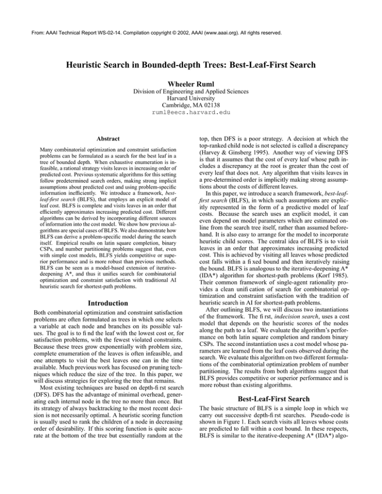
From: AAAI Technical Report WS-02-14. Compilation copyright © 2002, AAAI (www.aaai.org). All rights reserved.
Heuristic Search in Bounded-depth Trees: Best-Leaf-First Search
Wheeler Ruml
Division of Engineering and Applied Sciences
Harvard University
Cambridge, MA 02138
ruml@eecs.harvard.edu
Abstract
Many combinatorial optimization and constraint satisfaction
problems can be formulated as a search for the best leaf in a
tree of bounded depth. When exhaustive enumeration is infeasible, a rational strategy visits leaves in increasing order of
predicted cost. Previous systematic algorithms for this setting
follow predetermined search orders, making strong implicit
assumptions about predicted cost and using problem-specific
information inefficiently. We introduce a framework, bestleaf-first search (BLFS), that employs an explicit model of
leaf cost. BLFS is complete and visits leaves in an order that
efficiently approximates increasing predicted cost. Different
algorithms can be derived by incorporating different sources
of information into the cost model. We show how previous algorithms are special cases of BLFS. We also demonstrate how
BLFS can derive a problem-specific model during the search
itself. Empirical results on latin square completion, binary
CSPs, and number partitioning problems suggest that, even
with simple cost models, BLFS yields competitive or superior performance and is more robust than previous methods.
BLFS can be seen as a model-based extension of iterativedeepening A*, and thus it unifies search for combinatorial
optimization and constraint satisfaction with traditional AI
heuristic search for shortest-path problems.
Introduction
Both combinatorial optimization and constraint satisfaction
problems are often formulated as trees in which one selects
a variable at each node and branches on its possible values. The goal is to find the leaf with the lowest cost or, for
satisfaction problems, with the fewest violated constraints.
Because these trees grow exponentially with problem size,
complete enumeration of the leaves is often infeasible, and
one attempts to visit the best leaves one can in the time
available. Much previous work has focused on pruning techniques which reduce the size of the tree. In this paper, we
will discuss strategies for exploring the tree that remains.
Most existing techniques are based on depth-first search
(DFS). DFS has the advantage of minimal overhead, generating each internal node in the tree no more than once. But
its strategy of always backtracking to the most recent decision is not necessarily optimal. A heuristic scoring function
is usually used to rank the children of a node in decreasing
order of desirability. If this scoring function is quite accurate at the bottom of the tree but essentially random at the
top, then DFS is a poor strategy. A decision at which the
top-ranked child node is not selected is called a discrepancy
(Harvey & Ginsberg 1995). Another way of viewing DFS
is that it assumes that the cost of every leaf whose path includes a discrepancy at the root is greater than the cost of
every leaf that does not. Any algorithm that visits leaves in
a pre-determined order is implicitly making strong assumptions about the costs of different leaves.
In this paper, we introduce a search framework, best-leaffirst search (BLFS), in which such assumptions are explicitly represented in the form of a predictive model of leaf
costs. Because the search uses an explicit model, it can
even depend on model parameters which are estimated online from the search tree itself, rather than assumed beforehand. It is also easy to arrange for the model to incorporate
heuristic child scores. The central idea of BLFS is to visit
leaves in an order that approximates increasing predicted
cost. This is achieved by visiting all leaves whose predicted
cost falls within a fixed bound and then iteratively raising
the bound. BLFS is analogous to the iterative-deepening A*
(IDA*) algorithm for shortest-path problems (Korf 1985).
Their common framework of single-agent rationality provides a clean unification of search for combinatorial optimization and constraint satisfaction with the tradition of
heuristic search in AI for shortest-path problems.
After outlining BLFS, we will discuss two instantiations
of the framework. The first, indecision search, uses a cost
model that depends on the heuristic scores of the nodes
along the path to a leaf. We evaluate the algorithm’s performance on both latin square completion and random binary
CSPs. The second instantiation uses a cost model whose parameters are learned from the leaf costs observed during the
search. We evaluate this algorithm on two different formulations of the combinatorial optimization problem of number
partitioning. The results from both algorithms suggest that
BLFS provides competitive or superior performance and is
more robust than existing algorithms.
Best-Leaf-First Search
The basic structure of BLFS is a simple loop in which we
carry out successive depth-first searches. Pseudo-code is
shown in Figure 1. Each search visits all leaves whose costs
are predicted to fall within a cost bound. In these respects,
BLFS is similar to the iterative-deepening A* (IDA*) algo-
BLFS(root)
1. Visit a few leaves
2. Nodes-desired ← number of nodes visited so far
3. Loop until time runs out:
4.
Double nodes-desired
5.
Estimate cost bound that visits nodes-desired nodes
6.
Call BLFS-expand(root, bound)
BLFS-expand(node, bound)
7. If leaf(node), visit(node)
8. else, for each child of node:
9.
If best-completion(child) ≤ bound
10.
BLFS-expand(child, bound)
number of nodes. In the implementation tested below, this
was accomplished by instead predicting, given a cost bound,
the number of nodes that would be visited if that bound were
used. A bisection-style search was then performed over possible cost bounds, searching for one that would yield, according to the model, approximately the desired number of
nodes.
The basic BLFS framework is remarkably simple. In the
remainder of this paper, we will demonstrate its power and
flexibility by instantiating the framework using two different
cost models. The first model we will consider is a static one
that is specified before the search begins.
BLFS with a Fixed Model: Indecision Search
Figure 1: Simplified pseudo-code for best-leaf-first search.
rithm for shortest-path problems. IDA* controls expansion
of a node n using a prediction of the cost of the best path
to the nearest goal that goes through n. Analogously, BLFS
uses the predicted cost of the best leaf below n. This allows
the algorithm to avoid descending into any subtree that does
not contain a leaf we wish to visit on this iteration (step 9).
However, BLFS uses an explicit representation of its predictive model, rather than a black-box function suppled by
the user, as in IDA*. Being able to choose a simple model
leads to two important advantages over IDA*. First, we can
choose a model that will give consistent predictions. That is
to say, we can ensure that the minimum-cost child of every
branching node has the same evaluation as its parent. This
enforces the semantics tying the value of a node to its best
descendant leaf. Having a consistent prediction function
means that BLFS is certain to reach leaves on every iteration,
never expanding a node unnecessarily and never overlooking
a node that has a descendant within the cost bound. (In practice, one could also achieve the first behavior by forcing the
search to expand the best child.) The second advantage that
BLFS enjoys over IDA* is that the cost bound can be updated optimally. Because the predicted costs are generated
by a known model, we can choose cost bounds that can be
expected to cause twice as many nodes to be visited as on
the previous iteration (step 5). By approximately doubling
the number of nodes visited on each iteration, BLFS limits
its overhead to a factor of less than three in the worst-case
situation in which the entire tree must be searched.
IDA* itself performs poorly on optimization problems for
two reasons. As a shortest-path algorithm, it is typically
used with an underestimating node evaluation function. This
causes the algorithm to visit an enormous number of internal nodes before reaching its first leaf. Because the node
evaluations depend on operator costs defined by the problem
domain, rather than by a known model, it is also difficult to
update the cost bound correctly. IDA* either has enormous
overhead, visiting few new nodes per iteration, or simulates
DFS, visiting all leaves in one giant iteration.
To summarize, the BLFS leaf model must support two
operations. The first is to predict, given a search node, the
lowest cost of any leaf below it. The second is to estimate
the cost bound that will cause the algorithm to visit a desired
As mentioned in the introduction, heuristic child ranking is
often used to guide tree search. Most such ranking functions
return a numerical score for each child, although the precise
semantics of this score varies. The first cost model we will
consider is based on these scores. We will assign each child
a cost based on how much worse its score is than the score
of the best child. If the child scores are s0 , . . . , sb , child
i has a cost of si − s0 . Furthermore, we will assume that
the cost of a leaf is simply the maximum of the costs of the
nodes along its path from the root. This is a generalization
of iterative broadening (Ginsberg & Harvey 1992), which
assumes that the cost of a leaf reflects the maximum rank
of any child along its path. Another way to think about this
cost model is that the cost of a node reflects how decisively
the heuristic score separated it from the best child. Paths
involving nodes for which the heuristic was only mildly indecisive in its ranking will be explored earlier in the search
than those involving nodes whose scores were much worse.
For this reason, we can call this instantiation of BLFS indecision search.
It is easy to support the operations needed for BLFS using this cost model. Because the preferred child is always
free, the predicted cost of the best leaf below any node is
just the maximum cost of any node encountered enroute to
the node itself. To predict the number of nodes visited for
a given cost bound, we assume independence and estimate
the average expected branching factor at each level of the
tree. The branching factor depends on the number of children at each level whose costs we expect to fall below the
cost bound. Although we probably do not know all of the
costs we will see, we will have seen many of them during
the previous iteration of indecision search. Recall that each
iteration explores a superset of the previous one, and that all
of the child scores at each node of the previous search will
have been computed in order to guide that search (step 9).
We will use these scores as samples to estimate the probability distribution over possible costs for each child rank
at each level of the tree. In the experiments reported here,
these estimated distributions were represented as histograms
(see Ruml (2002) for more details on this estimation). Note
that, although we estimate on-line the node costs we expect
to observe in the tree, the underlying leaf cost model itself is
fixed as exactly the maximum node cost in the path, and is
not adjusted during search. The initial iteration of the algorithm (step 1) visits all leaves of predicted cost zero. There
n
11
13
15
17
19
21
Fraction of Problems Solved
0.8
0.6
DFS
7,225
888,909
∞
∞
∞
∞
Indec.
188
298
402
648
908
1,242
ILDS
183
303
621
1,047
1,609
2,812
DDS
206
357
642
1,176
1,852
3,077
Indec / ILDS
1.03
.983
.647
.619
.564
.442
0.4
Indecision
ILDS (bottom)
ILDS (top)
DDS
DFS
0.2
2.7
3.0
3.3
3.6
Table 1: The number of nodes generated to solve latin square
completion problems, represented by the 95th percentile of
the distribution across random instances.
3.9
Log10(Nodes Generated)
Figure 2: Distribution of search times when completing 21×
21 latin squares with 30% of the cells preassigned.
may be multiple such leaves, depending on how many ties
there are for minimum child score.
Other schemes in addition to iterative broadening can be
viewed as approximations to indecision search. The randomized restarting technique of Gomes, Selman, & Kautz
(1998) and the GRASP methodology of Feo & Resende
(1995) both randomly permute, between iterations of search,
all children whose scores are within a specified distance
from the preferred child. These techniques depend on an
equivalence parameter that must be tuned using pilot experiments, and restarting also depends on a time limit parameter.
Also, because they regard closely-scoring children as equivalent, these techniques throw away information that can be
systematically exploited by indecision search.
Evaluation
We can use constraint satisfaction problems to evaluate indecision search, as they are commonly solved using a heuristic
scoring function to rank children in increasing order of ‘constrainingness.’ We will examine two domains: latin square
completion and random binary CSPs.
Latin Squares A latin square is an n by n array in
which each cell has one of n colors. Each row and column must contain each color exactly once. Gomes & Selman (1997) proposed the completion of partially-filled latin
squares as a challenging benchmark problem. We used
forward-checking, choosing variables to assign according to
the most-constrained variable heuristic of Brélaz (1979) and
ranking values according to the logarithm of the promise
heuristic of Geelen (1992). Following Meseguer & Walsh
(1998), we used 1,000 latin squares, each with 30% of the
cells assigned, filtering out any unsatisfiable problems. We
tested depth-first search (DFS), two version of Korf’s improved limited discrepancy search (ILDS, Korf, 1996), one
taking discrepancies at the top first and the other taking them
at the bottom first, depth-bounded discrepancy search (DDS,
Walsh, 1997), and indecision search.
The performance of the algorithms is shown in Figure 2
in terms of the fraction of problems solved within a given
number of node generations. Small horizontal error bars
mark 95% confidence intervals around the means. Depthfirst search was limited to 10,000 nodes per problem, hence
its mean is a lower bound. From the figure, we see that
25% of the problems were solved by visiting a single leaf
(the greedy solution). Depth-first search is notoriously brittle and becomes hopeless lost on many problems (Gomes et
al. 2000). The discrepancy search algorithms immediately
retreat to the root. Indecision search first explores all ties,
which may occur at intermediate levels of the tree, and it
solves all the problems within 4,000 nodes (note the logarithmic scale). Similar behavior was observed on smaller instances, although the advantage of indecision search over the
discrepancy methods seemed to increase as problems grew
larger (Table 1).
Binary CSPs Binary CSPs have received much attention
in the literature and were used by Meseguer & Walsh (1998)
to evaluate DDS and interleaved depth-first search (IDFS).
They tested on satisfiable problems of the hn, m, p1 , p2 i
type. These problems have n variables, each with m possible values. Exactly p1 n(n − 1)/2 of the possible pairs of
variables are constrained and exactly p2 m2 of the possible
value combinations are disallowed for each of those pairs.
As p2 increases from .3 toward 0.36, the constraints become
tighter and the problems become more difficult to solve, exposing differences in performance between the algorithms.
Following Meseguer & Walsh, we used the three classes
h30, 15, .4, p2i, h50, 12, .2, p2i, and h100, 6, .06, p2i, generating 100 instances at various tightness values. We will use
the same heuristics as employed above with latin squares.
As with latin squares, there is enormous variance in the
number of nodes generated by each algorithm within each
set of 100 similar instances. We focus on the upper tail of
the distribution because it essentially controls the expected
value. We avoid the maximum, as it is subject to sampling
error. Table 2 shows the 95th percentile of each distribution.
Problem classes are identified by number of variables and
tightness value. At very low tightness (not shown), problems are easy and DFS is sufficient. DFS always exhibited
the best median performance, but as tightness increases the
tail of its distribution grew rapidly. Indecision search is either the best or within 25% of the best in every instance class
except h30, .360i. This isolated case of poor performance
seems to be due to inaccurate cost bound estimation, causing indecision search to visit only a constant number of new
DFS
241
1,119
4,881
42,025
103,878
164
1,450
3,156
22,852
352,788
110
31,910
208,112
Indec.
391
884
4,501
28,294
536,716
320
984
3,410
28,630
387,432
676
3,344
70,664
ILDS
456
1,122
5,862
30,996
309,848
358
1,271
6,389
52,491
554,036
646
4,012
127,712
DDS
424
1,115
8,014
100,387
1,642,806
408
1,301
12,790
187,856
3,546,588
826
11,845
2,048,320
-4
DDS
ILDS
BLFS
DFS
-5
Log10(Difference)
hn, p2 i
30, .307
30, .320
30, .333
30, .347
30, .360
50, .306
50, .319
50, .333
50, .347
50, .361
100, .306
100, .333
100, .361
-6
-7
200,000
400,000
600,000
800,000
1,000,000
Nodes Generated
Table 2: The number of nodes needed to solve binary CSPs
from various classes. Each number is the 95th percentile of
the distribution over instances of that class.
nodes per iteration. Supplying feedback to the estimation
process should allow automated detection and correction of
such errors.
Experiments were also performed using a cost model that
predicted the cost of a leaf to be the sum of the child costs
along its path, rather than just the maximum. This model
seemed to perform similarly, and is more cumbersome to
manipulate, so we omit further discussion of it (see Ruml
(2002) for details).
BLFS with a Learned Model
In some domains, the child ranking function does not return
a quantitative score and the only information that is readily
available to guide search is the costs of the leaves that have
been visited. Following Ruml (2001a), we will use these
observed costs to estimate the cost of taking a discrepancy
at each level of the tree. More precisely, we will use a cost
model that assumes that the cost of a leaf is the sum of the
costs of the edges taken to reach it, and we will assume that
the cost of an edge depends only on its depth and its rank
in the sorted list of children. A tree of depth d and branching factor b requires db parameters, one for each child rank
at each level. This generalizes DFS, ILDS, DDS, and interleaved DFS(Meseguer 1997), as their search orders can be
simulated by the appropriate parameter settings.
Because these edge costs will vary depending on the problem, we will estimate them during the search. In step 1 of
BLFS, we will visit 10 random leaves. Each path forms a linear equation in the parameters of the model. After visiting
each leaf (in either step 1 or 7), we can update the parameters using on-line linear regression (Murata et al. 1997).
To help ensure that the current cost bound yields the predicted number of nodes, a static copy of the model is made
at the start of each iteration to guide the search. To further
aid learning, the costs estimated in the experiments below
were further constrained at the start of each iteration to be
increasing with child rank at each depth. (In other words, it
was assumed that the underlying ranking function was helpful rather than deceptive.)
Figure 3: Greedy partitioning of 128 numbers
This cost model also easily supports the operations required for BLFS. The cost of the best leaf in any subtree
is just the sum of the edges traversed so far plus the sum of
the costs of the cheapest options at each of the remaining
levels. These optimal completions can be precomputed at
the start of each iteration. To estimate the number of nodes
that will be visited for a given bound, we just estimate the
branching factor at each level, as for indecision search. We
can consider the cost bound to be an allowance that is spent
as we descend the tree. By estimating the distribution of
allowance values expected at each level of the tree, we can
estimate how many children whose best completion will be
affordable at that level. (As in indecision search, these distributions are manipulated as histograms, as described in the
appendix.) At the root, the allowance distribution is a spike
at the given cost bound. The distribution of allowance at the
next level is just the sum, over the possible children, of the
portion of the current distribution that falls above the best
completion cost for that child, translated toward zero by that
cost. Each distribution in the sum is weighted by the proportion of the probability that survived the truncation. (See
Ruml (2002) for more details.)
Evaluation
We evaluated the algorithm on two different formulations
of the combinatorial optimization problem of number partitioning. The objective is to divide a given set of numbers into two disjoint groups such that the difference between the sums of the two groups is as small as possible.
It has been used by many authors as a challenging benchmark for search algorithms (Johnson et al. 1991; Korf 1996;
Walsh 1997; Ruml 2001a). Following Ruml, we encouraged
difficult search trees by using instances with many digits of
precision (44 digits for 128-number problems and 82 digits for 256-number problems). Arbitrary precision integer
arithmetic was used in the implementation, and results were
normalized as if the original numbers had been between 0
and 1. The logarithm of the partition difference was used as
the leaf cost.
The first formulation of partitioning as a search is a
DDS
ILDS
BLFS
DFS
DDS
DFS
ILDS
BLFS
-12.8
-4
Log10(Difference)
Log10(Difference)
-2
-6
-13.2
-13.6
-14.0
-8
400,000
800,000
1,200,000
1,600,000
2,000,000
Nodes Generated
800,000
1,200,000
1,600,000
2,000,000
Nodes Generated
Figure 4: Greedy partitioning of 256 numbers
Figure 6: CKK representation for partitioning 256 numbers
DDS
DFS
BLFS
ILDS
-10.4
follows ILDS in this new search space where it is superior.
Looking across instance sizes, we see that the advantage of
BLFS increases as problems become larger. For large number partitioning problems, BLFS in the CKK search space is
the best algorithm known.
-10.8
Log10(Difference)
400,000
-11.2
Discussion
-11.6
-12.0
200,000
400,000
600,000
800,000
1,000,000
Nodes Generated
Figure 5: CKK representation for partitioning 128 numbers
straightforward greedy encoding in which the numbers are
sorted in descending order and then each decision places the
largest remaining number in a partition, preferring the partition with the currently smaller sum. Figures 3 and 4 compare the performance of BLFS with DFS, ILDS, and DDS.
Error bars in the figures indicate 95% confidence intervals
around the mean. Although BLFS does not surpass DFS in
this search space, looking across the two instance sizes indicates that it consistently tracks DFS as the problem size
increases, unlike ILDS and DDS, whose solution quality actually decreases on larger problems.
A more sophisticated representation for number partitioning was suggested by Korf (1995), based on the heuristic of
Karmarkar and Karp (1982). The essential idea is to postpone the assignment of numbers to particular partitions and
merely constrain pairs of number to lie in either different
bins or the same bin. Numbers are considered in decreasing
order and constrained sets are reinserted in the list according to the remaining difference they represent. Figures 5 and
6 compare the performance of BLFS with DFS, ILDS, and
DDS. BLFS tracked DFS in the greedy search space but now
BLFS is very similar to the iterative-deepening A* (IDA*)
algorithm for shortest-path problems, but depends on an explicit cost model (see Table 3). Because the cost model is explicit, the cost bound can be updated efficiently even when
few nodes have the same cost, unlike with IDA*. For efficiency, the cost model should give consistent predictions.
Happily, such a model can easily be learned, even during the
search it is intended to guide. The use of an additive cost
model is inherent in the shortest-path problems for which
IDA* was designed, but it is merely a convenient route to
consistency for BLFS. Many optimization problems, such
as number partitioning, have no inherent notion of operator
cost. What matters is the expected cost of taking a heuristically less-preferred child.
This unification of traditional AI heuristic search with
bounded-depth tree search clarifies some of the confusion
attendant to the term ‘heuristic search’, which is often applied to both shortest-path algorithms with a heuristic costto-goal estimate (h(n)) and also to procedures like DFS with
a node ordering function. BLFS makes it clear that a node
ordering function is just a rough indicator of the cost of the
best leaf in the subtree, and by adhering to this semantics, it
approximates a rational search order.
BLFS is also related to previous work on learning for
search. This was explored in the context of improvement
search, as opposed to tree search, by Baluja & Davies (1998)
and Boyan & Moore (1998). Techniques for managing the
trade-off between time and expected solution improvement
are orthogonal to BLFS, and could be applied on top of it.
Mayer (1994) and Hansson (1998) have done preliminary
work in this direction.
In practice, the main drawback of BLFS is its runtime
f (n) semantics
desired f (n) property
f (n) non-overestimating
f (n) non-underestimating
f (n) source
g(n) source
h(n) source
additive model
updating bound
BLFS
best leaf below n
consistent
correctness
efficiency
from user or learned
not necessary
not necessary
convenient
estimation
rational
IDA*
best path through n
non-overestimating
optimality
efficiency
= g(n) + h(n)
from problem
from user
required
add optimal
Table 3: A comparison of BLFS and IDA*.
overhead, which can be noticeable if the search is short.
The most expensive operation is the cost bound estimation, which is done a logarithmic number of times. For the
number partitioning experiments reported here, for example,
overheads of 20–30% were not uncommon in our prototype
implementation. Further engineering work is needed to determine how small this overhead can be made.
Possible Extensions
It would be very interesting to explore other models besides those investigated here. It should be straightforward to
combine on-line learning of weights with the heuristic child
scores used in indecision search. This would relax the assumption that heuristic scores are strictly comparable across
levels. Multiple models could be trained simultaneously and
the one with the lowest error on the previous iteration could
be used to guide search. By constraining adjacent costs to
be similar, fewer parameters would be needed in the model,
and it might be feasible to consider learning models for both
value choice and variable choice (Ruml 2001b).
BLFS currently does not take into account the uncertainty
in its cost model or the possible benefits of visiting a leaf
predicted to be poor. A drastically misestimated cost can
cause the search to avoid the corresponding edge and fail to
correct the estimate. One way to remedy this would be to
use as a node evaluation the probability that the node leads
to the optimal leaf. This could be computed from a child
cost model by estimating variance and assuming normality,
following Ruml (2001a). The cost bound on each iteration
would become a probability bound. This seems similar to
the methods proposed by Bedrax-Weiss (1999), although her
algorithm was trained and scheduled off-line. Active learning under a known deadline is another possible direction.
Conclusions
We introduced best-leaf-first search (BLFS), a new framework for searching the bounded-depth trees that arise in
combinatorial optimization and constraint satisfaction problems. BLFS generalizes previous work and represents the
first successful rational approach to search for this setting.
Empirical results show that, even with simple cost models,
BLFS performs well on a variety of synthetic benchmark
problems, yielding results competitive with or superior to
the best previous method for each problem. Its robustness
is unparalleled. It retains completeness while adapting online to individual problem instances and it uses an explicit
model of its assumptions. Perhaps most importantly, BLFS
shows how search for combinatorial optimization and constraint satisfaction can be viewed from a perspective similar
to that of traditional heuristic search for shortest-path problems, as the strategy of a rational agent trying to efficiently
take advantage of heuristic information for problem-solving.
Acknowledgments
Stuart Shieber and the Harvard AI Research Group gave numerous helpful suggestions. This work was supported in
part by NSF grants CDA-94-01024 and IRI-9618848.
References
Baluja, S., and Davies, S. 1998. Fast probabilistic modeling for combinatorial optimization. In Proceedings of
AAAI-98.
Bedrax-Weiss, T. 1999. Optimal Search Protocols. Ph.D.
Dissertation, University of Oregon, Eugene.
Boyan, J. A., and Moore, A. W. 1998. Learning evaluation
functions for global optimization and boolean satisfiability.
In Proceedings of AAAI-98.
Brélaz, D. 1979. New methods to color the vertices of a
graph. Communications of the ACM 22(4):251–256.
Feo, T. A., and Resende, M. G. C. 1995. Greedy randomized adaptive search procedures. Journal of Global
Optimization 6:109–133.
Geelen, P. A. 1992. Dual viewpoint heuristics for binary
constraint satisfaction problems. In Neumann, B., ed., Proceedings of ECAI-92, 31–35.
Ginsberg, M. L., and Harvey, W. D. 1992. Iterative broadening. Artificial Intelligence 55:367–383.
Gomes, C. P., and Selman, B. 1997. Problem structure in
the presence of perturbations. In Proceedings of AAAI-97,
221–226.
Gomes, C. P.; Selman, B.; Crato, N.; and Kautz, H.
2000. Heavy-tailed phenomena in satisfiability and constraint satisfaction problems. Journal of Automated Reasoning 24:67–100.
Gomes, C. P.; Selman, B.; and Kautz, H. 1998. Boosting
combinatorial search through randomization. In Proceedings of AAAI-98.
Hansson, O. 1998. Bayesian Problem-Solving Applied to
Scheduling. Ph.D. Dissertation, University of California,
Berkeley.
Harvey, W. D., and Ginsberg, M. L. 1995. Limited discrepancy search. In Proceedings of IJCAI-95, 607–613.
Morgan Kaufmann.
Johnson, D. S.; Aragon, C. R.; McGeoch, L. A.; and
Schevon, C. 1991. Optimization by simulated annealing: An experimental evaluation; Part II, graph coloring
and number partitioning. Operations Research 39(3):378–
406.
Karmarkar, N., and Karp, R. M. 1982. The differencing
method of set partitioning. Technical Report UCB/CSD
82/113, Computer Science Division, University of California, Berkeley.
Korf, R. E. 1985. Depth-first iterative-deepening: An
optimal admissible tree search. Artificial Intelligence
27(1):97–109.
Korf, R. E. 1995. From approximate to optimal solutions:
A case study of number partitioning. In Proceedings of
IJCAI-95.
Korf, R. E. 1996. Improved limited discrepancy search. In
Proceedings of AAAI-96, 286–291. MIT Press.
Mayer, A. E. 1994. Rational Search. Ph.D. Dissertation,
University of California, Berkeley.
Meseguer, P., and Walsh, T. 1998. Interleaved and discrepancy based search. In Proceedings of ECAI-98.
Meseguer, P. 1997. Interleaved depth-first search. In Proceedings of IJCAI-97, 1382–1387.
Murata, N.; Müller, K.-R.; Ziehe, A.; and Amari, S. 1997.
Adaptive on-line learning in changing environments. In
Mozer, M.; Jordan, M.; and Petsche, T., eds., Advances in
Neural Information Processing Systems 9 (NIPS-96), 599–
605. MIT Press.
Ruml, W. 2001a. Incomplete tree search using adaptive
probing. In Proceedings of IJCAI-01, 235–241.
Ruml, W. 2001b. Stochastic tree search: Where to put the
randomness? In Hoos, H. H., and Stützle, T. G., eds., Proceedings of the IJCAI-01 Workshop on Stochastic Search,
43–47.
Ruml, W. 2002. Adaptive Tree Search. Ph.D. Dissertation,
Harvard University.
Walsh, T. 1997. Depth-bounded discrepancy search. In
Proceedings of IJCAI-97.