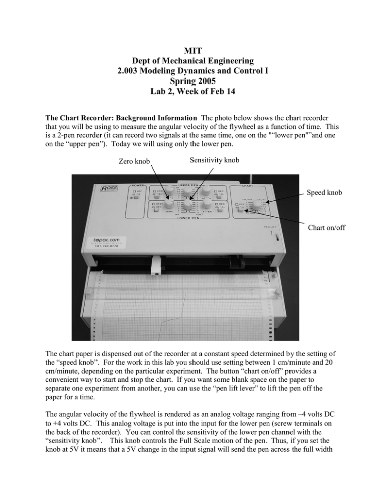
MIT
Dept of Mechanical Engineering
2.003 Modeling Dynamics and Control I
Spring 2005
Lab 2, Week of Feb 14
The Chart Recorder: Background Information The photo below shows the chart recorder
that you will be using to measure the angular velocity of the flywheel as a function of time. This
is a 2-pen recorder (it can record two signals at the same time, one on the "“lower pen"”and one
on the “upper pen”). Today we will using only the lower pen.
Zero knob
Sensitivity knob
Speed knob
Chart on/off
The chart paper is dispensed out of the recorder at a constant speed determined by the setting of
the “speed knob”. For the work in this lab you should use setting between 1 cm/minute and 20
cm/minute, depending on the particular experiment. The button “chart on/off” provides a
convenient way to start and stop the chart. If you want some blank space on the paper to
separate one experiment from another, you can use the “pen lift lever” to lift the pen off the
paper for a time.
The angular velocity of the flywheel is rendered as an analog voltage ranging from –4 volts DC
to +4 volts DC. This analog voltage is put into the input for the lower pen (screw terminals on
the back of the recorder). You can control the sensitivity of the lower pen channel with the
“sensitivity knob”. This knob controls the Full Scale motion of the pen. Thus, if you set the
knob at 5V it means that a 5V change in the input signal will send the pen across the full width
of the chart. For this session you will probably want to choose sensitivities between 1V and 5.
You can also turn the “zero knob” to change the location of the pen which corresponds to zero
speed. Most convenient is to locate the zero near the right hand side of the paper.
Please make sure that the following buttons and knobs are in their “default” positions:
·
·
·
The button marked “Stby/Rec” should be down.
The button marked “Rec/Cal” should be up.
The knob marked “Atten” should remain all the way counterclockwise (there is a
“detent/click” at this position”)
Laboratory
1) Calibrate the speed measurement. Make sure that all the magnets are in their storage
positions (not under the flywheel). Set the lower pen chart sensitivity to 2V full scale deflection
and make sure the pen is zeroed near the right had side of the paper. Give the flywheel a spin so
as to cause the pen to move MOST of the way to the left on the paper. Measure the angular
velocity of the flywheel using a stop watch or second hand. Calculate a calibration constant in
units like [radians/sec/volt]. Test the linearity of the measurement by repeating at a much lower
speed. HINT: you only need a value that is accurate within 10%.
Also, make sure you write on your chart paper to record the speed and sensitivity for each
measurement throughout the lab.
2) Eddy-Current Damping Take the magnet which is not on a standoff and run it by hand up
and down the provided copper slab at different speeds and at different distances. Let the magnet
slide down the copper as a mass sliding down an inclined plane. Change the angle of the plane
and try again. Explain what you observe.
3) Free-response of a First order System. Put one magnet under the flywheel (centered under
the copper rim). Spin the flywheel up to a speed of about 1 rev/sec by hand and record the decay
of the speed on the chart recorder. How close is your plot to what you expect from a linear firstorder system? Where does it deviate from this idealized behavior (if at all)? Estimate the time
constant of the system from the plot.
If you were to repeat this for a much higher initial speed of the flywheel (say twice as high,
would you expect the time constant to be the same, lower or higher? Do the experiment and
discuss.
Estimate the value of the damping coefficient, b. What are the units?
4) Free Response with More Damping. Put a total of two magnets under the flywheel. What
do you expect the time constant of this system to be? Run the experiment and measure the time
constant.
5) Driven response of a first order system. With one magnet under the flywheel, wind the
string attached to one weight and around the pulley and attach one brass weight as shown in the
photo below (the mass of the weight is about 0.11 kg) . Record the speed as the flywheel comes
up to speed from a standstill. This data actually allows for two independent measurements of the
Damping Constant – discuss. Measure/deduce the damping constant in the two ways and
compare the results. (Note: for the pulley/string combination use a diameter of 13mm, which
accounts for the string thickness).
Weight
hanging over
the side of
counter
6) More Driven Response. Add a second weight, by hanging it from the string over the first
weight. Predict the behavior that you expect by sketching on the chart paper itself – mark it as
prediction. Run the experiment and compare your prediction with observations.
7) Free response with no Damping. Remove all magnets from under flywheel. If you were
to spin the flywheel up to speed and let it coast, what do you expect the speed would like as a
function of time. Sketch it out and provide approximate scaling on the time axis. Run the
experiment. What is the shape of the response? What type of damping or friction is present?
What are the magnitudes and units?
8) (extra credit) Move one magnet into a position such that the free response of the system
shows aspects of BOTH linear damping and Coulomb friction. Explain what you are seeing.
9) (extra credit) In #5 above, we ignored the contribution of the falling weight to the dynamics
of the system. How large a contribution is it?
Lab Report (In this lab section you will provide a set of plots per group, since it is hard to
reproduce extra copies of the chart recorder plots)
Your group’s lab report should consist of the following: 1) Your chart paper with marking for speed and sensitivity as well as notations about which question each recording pertains to. List all group members on the sheet.
2) A table or other concise listing of the specific numerical results that you measured and calculated. 3) Individual lab responses to questions.