Can we reconstruct Localized Features from
Non-Local Observations?
the role of observation and background errors
Olaf Stiller
Deutscher Wetterdienst, Data Assimilation Unit, Frankfurter Str. 135, Offenbach, Germany
(1) Can the DA system represent localised features?
(2) If observation errors were negligible:
The Pseudo-Inverse Solution (PI)
• Most modern DA systems determine the analysis increments
sensitivity
x a = Xa − Xb
General solution for the cost function minimum xa (of Eq.(1)):
functions
h
xa = B−1 + HT R−1H
via a costfunction
o
1 n T −1
x B x + [y − Hx]T R−1 [y − Hx]
J(x) =
2
i−1
HT R−1y
(2)
For vanishing obs errors (R →h 0) this iyields the Pseudo Inverse (PI)
−1
T
exists)
(assume for the moment that HBH
(1)
• Many observations (particularly satellite radiances) are strongly
nonlocal
h
x̌a = BHT HBHT
• DA systems have to deal with strongly localised features like
cloud tops, inversions, etc.
with
i−1
y
(3)
Hi x̌a = yi .
The PI
Question: Can the costfunction minimum describe such localised features?
Assume: Observations are locally very dense
(as true for IR radiances from hyperspectral sounders)
• is consistent with all observations y = {y1, y2, .., yp}
• describes localised features as detailed as the density of observations allows
• potentially amplifies noise
(3) Finite observation errors degrade
representation of localised feature
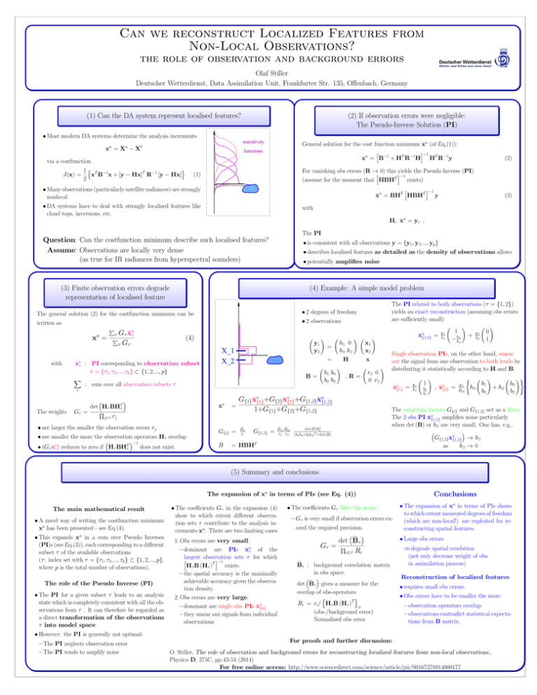
(4) Example: A simple model problem
The general solution (2) for the costfunction minimum can be
• 2 degrees of freedom
written as
• 2 observations
a
x =
with
a
x̌τ
X
P
a
τ Gτ x̌τ
P
τ Gτ
(4)
: PI corresponding to observation subset
τ = {τ1, τ2, .., τk } ⊂ {1, 2, .., p}
y1
y2
X_1
X_2
!
=
=
B=
: sum over all observation subsets τ
b1 b0
b0 b2
h1 0
h0 h2
H
!
The PI related to both observations (τ = {1, 2})
yields an exact reconstruction (assuming obs errors
are sufficiently small)
!
x1
x2
x
!
r1 0
0 r2
,R=
x̌a{1,2}
!
The weights
Gτ =
det Hτ BHTτ
Q
j∈τ
rj
xa
• are larger the smaller the observation errors rj
• are smaller the more the observation operators Hτ overlap
• (Gτ x̌aτ )
reduces to zero if
Hτ BHTτ
−1
does not exist.
G{i} =
B̂
B̂ii
ri
G{1,2} =
1
− hh20
+
y2
h2
0
1
!
Single observation PIs, on the other hand, smear
out the signal from one observation to both levels by
distributing it statistically according to H and B.
x̌a{1}
τ
G{1}x̌a{1}+G{2}x̌a{2}+G{1,2}x̌a{1,2}
=
1+G{1}+G{2}+G{1,2}
=
y1
h1
!
=
y1
h1
1
b0
b1
!
;
x̌a{2}
=
y2
B̂22
(
h0
b1
b0
!
+ h2
b0
b2
The weighting factors G{i} and G{1,2} act as a filter.
The 2 obs PI x̌a{1,2} amplifies noise particularly
when det (B) or h2 are very small. One has, e.g.,
det(B)h22
B̂11 B̂22
r1 r2 (b1h0+b0h2)2+det(B)
= HBHT
G{1,2}x̌a{1,2} → h2
as
h2 → 0
(5) Summary and conclusions
The expansion of xa in terms of PIs (see Eq. (4))
The main mathematical result
• A novel way of writing the costfunction minimum
xa has been presented - see Eq.(4).
• This expands xa in a sum over Pseudo Inverses
(PI)s (see Eq.(3)), each corresponding to a different
subset τ of the available observations
(τ : index set with τ = {τ1, τ2, .., τk } ⊂ {1, 2, .., p},
where p is the total number of observations).
The role of the Pseudo Inverse (PI)
• The PI for a given subset τ leads to an analysis
state which is completely consistent with all the observations from τ . It can therefore be regarded as
a direct transformation of the observations
τ into model space.
• The coefficients Gτ in the expansion (4)
show to which extent different observation sets τ contribute to the analysis increments xa. There are two limiting cases
1. Obs errors are very small:
– dominant are PIs x̌aτ of the
largest
observation
sets
τ
for
which
h
i
T −1
exists.
Hτ B (Hτ )
– the spatial accuracy is the maximally
achievable accuracy given the observation density.
2. Obs errors are very large:
– dominant are single obs PIs x̌a{k}
– they smear out signals from individual
observations
Conclusions
• The coefficients Gτ filter the noise.
– Gτ is very small if observation errors exceed the required precision.
f
det Bτ
Gτ = Q
i∈τ Ri
e : background correlation matrix
B
τ
in obs space.
e
det B
τ gives a measure for the
overlap of obs-operators
n
T
o
Ri = ri/ Hτ B (Hτ )
ii
(obs-/background error)
Normalised obs error
• The expansion of xa in terms of PIs shows
to which extent measured degrees of freedom
(which are non-local!) are exploited for reconstructing spatial features.
• Large obs errors
⇒ degrade spatial resolution
(not only decrease weight of obs
in assimilation process)
Reconstruction of localized features
• requires small obs errors.
• Obs errors have to be smaller the more
– observation operators overlap.
– observations contradict statistical expectations from B matrix.
• However: the PI is generally not optimal:
– The PI neglects observation error
– The PI tends to amplify noise
!)
For proofs and further discussion:
O. Stiller, The role of observation and background errors for reconstructing localized features from non-local observations.,
Physica D, 275C, pp.43-53 (2014)
For free online access: http://www.sciencedirect.com/science/article/pii/S0167278914000177