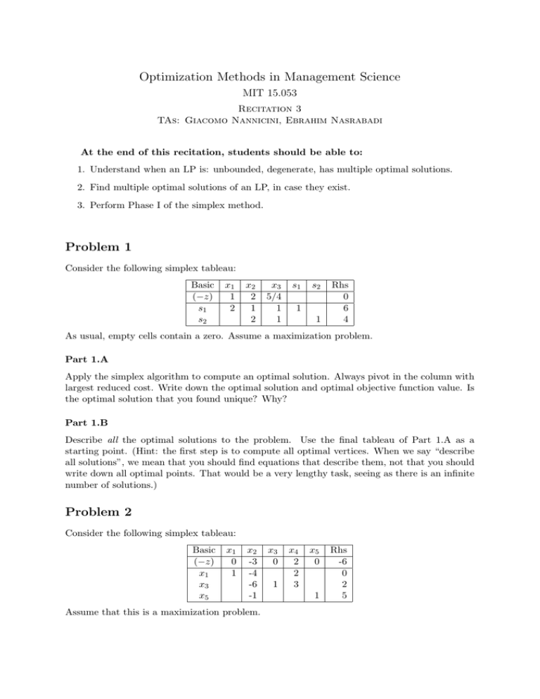
Optimization Methods in Management Science
MIT 15.053
Recitation 3
TAs: Giacomo Nannicini, Ebrahim Nasrabadi
At the end of this recitation, students should be able to:
1. Understand when an LP is: unbounded, degenerate, has multiple optimal solutions.
2. Find multiple optimal solutions of an LP, in case they exist.
3. Perform Phase I of the simplex method.
Problem 1
Consider the following simplex tableau:
Basic
(−z)
s1
s2
x1
1
2
x2
2
1
2
x3
5/4
1
1
s1
s2
1
1
Rhs
0
6
4
As usual, empty cells contain a zero. Assume a maximization problem.
Part 1.A
Apply the simplex algorithm to compute an optimal solution. Always pivot in the column with
largest reduced cost. Write down the optimal solution and optimal objective function value. Is
the optimal solution that you found unique? Why?
Part 1.B
Describe all the optimal solutions to the problem. Use the final tableau of Part 1.A as a
starting point. (Hint: the first step is to compute all optimal vertices. When we say “describe
all solutions”, we mean that you should find equations that describe them, not that you should
write down all optimal points. That would be a very lengthy task, seeing as there is an infinite
number of solutions.)
Problem 2
Consider the following simplex tableau:
Basic
(−z)
x1
x3
x5
x1
0
1
x2
-3
-4
-6
-1
Assume that this is a maximization problem.
x3
0
1
x4
2
2
3
x5
0
1
Rhs
-6
0
2
5
Part 2.A
What is the current basic feasible solution and its objective function value? Is the current bfs
degenerate?
Part 2.B
Perform one pivot. What is the new basic feasible solution and its objective function value? Did
anything change with respect to the previous bfs? And with respect to the previous tableau?
Part 2.C
The tableau that you obtained after Part 2.B is not optimal because some reduced cost is
positive. In fact, the problem is unbounded (why?). Give the equations describing a ray of the
feasible region along which the objective function can be increased indefinitely.
Problem 3
Consider the following LP:
max
⎫
x1 + 3x2
⎪
⎪
⎬
2x1 − 2x2 = 1
x1 + x2 ≥ 5 ⎪
⎪
⎭
x1 , x2 ≥ 0
(LP)
Observe that a basic feasible solution is not readily apparent. We want to perform Phase I of
the simplex method to find an initial basic feasible solution.
Part 3.A
Add surplus and artificial variables as needed to perform Phase I, then determine the Phase
I objective function. Write the resulting LP and the corresponding initial Phase I simplex
tableau. What is the basic feasible solution in this tableau?
Part 3.B
Perform two iterations of the simplex algorithm on the tableau obtained at the end of Part 3.A.
Is Phase I completed? If we now have a basic feasible solution for the original problem, explain
why and write the solution. If we do not have a basic feasible solution for the original problem,
explain why.
Problem 4
(Note: this problem is more difficult than the rest, and will require some serious thinking. You
will not be tested on Problem 4 in the upcoming quizzes, problem sets or midterms. However
it is very useful for understanding some subtleties of Phase I of the simplex method.)
Suppose that we have an LP with three nonnegative variables x1 , x2 , x3 to which we have
to apply Phase I of the simplex method to find an initial basic feasible solution. The artificial
variables are labeled s1 , s2 , s3 . After a few iterations of the simplex method in Phase I, we obtain
the following optimal tableau with an objective function value of zero, where b is a parameter
that will be specified later:
2
Basic
(−w)
x1
x2
s2
x1
x2
1
1
x3
-1
2
1
b
s1
-3
1
-3
1
s2
1
s3
-1
2
5
-1
Rhs
4
1
The artificial variable s2 is still basic, therefore we do not have a basis for the original problem.
But the objective value of Phase I is zero, therefore a bfs for the original problem exists. Our
goal is to find a basis to start Phase II of the simplex method.
Part 4.A
Assume b = −2. How do we proceed in this case? Determine a basis for the original problem
and the corresponding tableau that can be used to start Phase II (after restoring the original
objective function, which is not relevant for the purposes of this problem). (Hint: try to perform
a pivot to drive the artificial variable out of the basis; this pivot may be something that you
are normally not allowed to do, but notice that the basis is degenerate.)
Part 4.B
Assume b = 0. How do we proceed in this case? Determine a basis for the original problem and
the corresponding tableau that can be used to start Phase II restoring the original objective
function. (Hint: write down the equation corresponding to the last row of the tableau, and
observe that this is a linear combination of the original constraints. What does this row mean
in terms of the original equations?)
3
MIT OpenCourseWare
http://ocw.mit.edu
15.053 Optimization Methods in Management Science
Spring 2013
For information about citing these materials or our Terms of Use, visit: http://ocw.mit.edu/terms.