2.29 Numerical Fluid Mechanics
Spring 2015 – Lecture 12
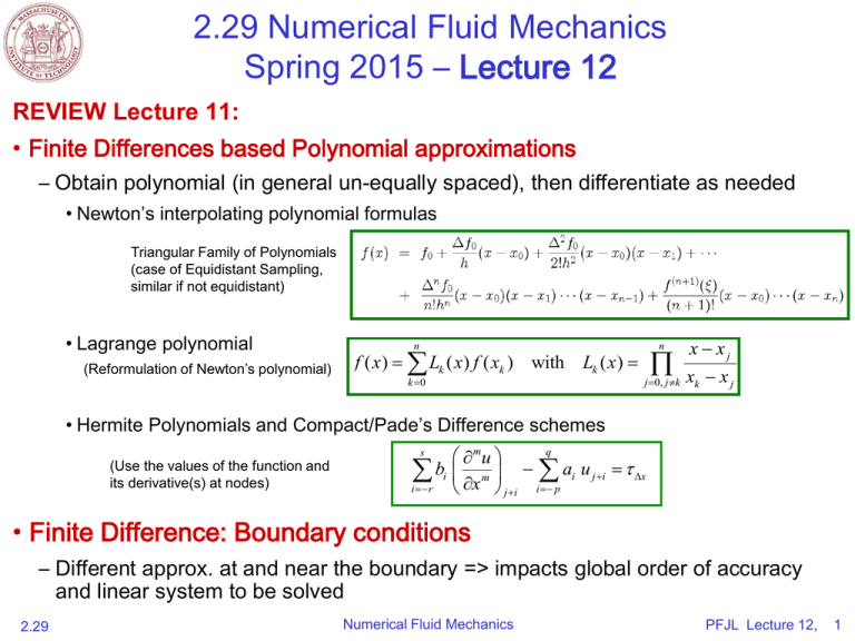
REVIEW Lecture 11:
• Finite Differences based Polynomial approximations
– Obtain polynomial (in general un-equally spaced), then differentiate as needed
• Newton’s interpolating polynomial formulas
Triangular Family of Polynomials
(case of Equidistant Sampling,
similar if not equidistant)
• Lagrange polynomial
(Reformulation of Newton’s polynomial)
n
x  xj
j 0, j k
xk  x j
n
f ( x )   Lk ( x ) f ( xk ) with Lk ( x ) 
k 0

• Hermite Polynomials and Compact/Pade’s Difference schemes
q
  mu 
ai u j i   x
 bi  x m   i
i  r

p

 j i
s
(Use the values of the function and
its derivative(s) at nodes)
• Finite Difference: Boundary conditions
– Different approx. at and near the boundary => impacts global order of accuracy
and linear system to be solved
2.29
Numerical Fluid Mechanics
PFJL Lecture 12,
1
2.29 Numerical Fluid Mechanics
Spring 2015 – Lecture 12
REVIEW Lecture 11:
• Finite Difference: Boundary conditions
– Different approx. at and near the boundary => impacts linear system to be
solved
• Finite-Differences on Non-Uniform Grids and Uniform Errors: 1-D
– If non-uniform grid is refined, error due to the 1st order term decreases faster
than that of 2nd order term
– Convergence becomes asymptotically 2nd order (1st order term cancels)
• Grid-Refinement and Error estimation
– Estimation of the order of convergence and of the discretization error
– Richardson’s extrapolation and Iterative improvements using Roomberg’s
algorithm
2.29
Numerical Fluid Mechanics
PFJL Lecture 12,
2
FINITE DIFFERENCES – Outline for Today
• Finite-Differences on Non-Uniform Grids and Uniform Errors: 1-D
• Grid Refinement and Error Estimation
• Fourier Analysis and Error Analysis
– Differentiation, definition and smoothness of solution for ≠ order of spatial operators
• Stability
– Heuristic Method
– Energy Method
– Von Neumann Method (Introduction) : 1st order linear convection/wave eqn.
• Hyperbolic PDEs and Stability
– Example: 2nd order wave equation and waves on a string
• Effective numerical wave numbers and dispersion
– CFL condition:
• Definition
• Examples: 1st order linear convection/wave eqn., 2nd order wave eqn., other FD schemes
– Von Neumann examples: 1st order linear convection/wave eqn.
– Tables of schemes for 1st order linear convection/wave eqn.
2.29
Numerical Fluid Mechanics
PFJL Lecture 12,
3
References and Reading Assignments
• Lapidus and Pinder, 1982: Numerical solutions of PDEs in
Science and Engineering. Section 4.5 on “Stability”.
• Chapter 3 on “Finite Difference Methods” of “J. H. Ferziger
and M. Peric, Computational Methods for Fluid Dynamics.
Springer, NY, 3rd edition, 2002”
• Chapter 3 on “Finite Difference Approximations” of “H. Lomax,
T. H. Pulliam, D.W. Zingg, Fundamentals of Computational
Fluid Dynamics (Scientific Computation). Springer, 2003”
• Chapter 29 and 30 on “Finite Difference: Elliptic and Parabolic
equations” of “Chapra and Canale, Numerical Methods for
Engineers, 2014/2010/2006.”
2.29
Numerical Fluid Mechanics
PFJL Lecture 12,
4
Grid-Refinement and Error estimation
• We found that for a convergent scheme, the discretization error ε is of
ˆ   ,
( ) 
0 , ˆxx (ˆ) 
0)
the form:
(recall:  
   O(x p )  R
where R is the remainder
• The degree of accuracy and discretization error can be estimated
between solutions obtained on systematically refined/coarsened grids
-True solution u can be expressed either as:
-Thus, the exponent p can be estimated:
u  ux   x p  R
u  u2 x   ' (2x ) p  R '
 u  u4 x 
p  log  2 x
 log 2
 ux  u2 x 
(need to eliminate u and then need 2 eqns. to eliminate both Δx and p, hence u4Δx )
-The discretization error on the grid Δx can be estimated by:  x 
ux  u2 x
2p 1
-Good idea: estimate p to check code. Is it equal to what it is supposed to be?
-When solutions on several grids are available, an approximation of higher
accuracy can be obtained from the remainder: Richardson Extrapolation!
2.29
Numerical Fluid Mechanics
PFJL Lecture 12,
5
Richardson Extrapolation and Romberg Integration
Richardson Extrapolation: method to obtain a third improved estimate of an
integral based on two other estimates
I(h)
Consider:
For two different grid space h1 and h2:
I
Trapezoidal Rule:

2
≈
h1
h2
h
(grid space)
Example
2
Assume:
)
From two O(h2),
we get an O(h4)!
Richardson Extrapolation:
2
2.29
Numerical Fluid Mechanics
PFJL Lecture 12,
6
Romberg’s Integration:
Iterative application of Richardson’s extrapolation
Romberg Integration Algorithm, for any order k
I(h)
For Order 2 (case of previous slide):
I
h2
k
Increasing order
1: O(h2)
2: O(h4)
a.
0.172800
1.068800
1.367467
b,.
0.172800
1.068800
1.484800
1.367467
1.623467
1.640533
0.172800
1.068800
1.484800
1.600800
1.367467
1.623467
1.639467
1.640533
1.640533
c.
Increasing
resolution
2.29
h
h1
j
3: O(h6)
Numerical Fluid Mechanics
4: O(h8)
1.640533
PFJL Lecture 12,
7
Romberg’s Differentiation:
Iterative application of Richardson’s extrapolation
‘Romberg’ Differentiation Algorithm, for any order k
D(h)
D
D
D
For Order 2 (as previous slide, but for differentiation):
D
D
h3
h
h1
k
Increasing order
1: O(h2)
2: O(h4)
a.
0.172800
1.068800
1.367467
b,.
0.172800
1.068800
1.484800
1.367467
1.623467
1.640533
0.172800
1.068800
1.484800
1.600800
1.367467
1.623467
1.639467
1.640533
1.640533
c.
Increasing
resolution
2.29
h2
j
4D2,1 – D1,1
3: O(h6)
Numerical Fluid Mechanics
4: O(h8)
1.640533
PFJL Lecture 12,
8
Fourier (Error) Analysis:
Definitions
• Leading error terms and discretization error estimates can be
complemented by a Fourier error analysis
• Fourier decomposition:
– Any arbitrary periodic function can be decomposed into its Fourier

components:
f ( x )   f k ei kx (k integer, wavenumber)
k 
2
i k x i m x
e
 e  2  km
(orthogonality property)
0
Using the orthog. property,
taking the integral/FT of f(x):
1
fk 
2
2

f ( x ) e  i k x dx
0
– Note: rate at which | fk | with |k| decays determine smoothness of f (x)
• Examples drawn in lecture: sin(x), Gaussian exp(-πx 2), multi-frequency functions,
etc
2.29
Numerical Fluid Mechanics
PFJL Lecture 12,
9
Fourier (Error) Analysis:
Differentiations
• Consider the decompositions:
f ( x) 


k 
fk e
i kx
f ( x, t ) 
or
• Taking spatial derivatives gives:
• Taking temporal derivatives gives:


k 
f k (t ) ei kx

n f
n i kx

f
(
t
)
ik
e



k
n
x
k 

r f
d r f k (t ) i kx
 
e
r
r
t
dt
k 
• Hence, in particular, for even or odd spatial derivatives:
2.29
n  2q

n  2q  1

ik   (1)q k 2 q
n
ik   i (1)q k 2 q1
n
Numerical Fluid Mechanics
(real)
(imaginary)
PFJL Lecture 12,
10
Fourier (Error) Analysis:
Generic equation
 f n f
 n
t
x
• Consider the generic PDE:
• Fourier Analysis:
f ( x, t ) 


k 

d f k (t ) i kx
n i kx
e

f
(
t
)
ik
e




k
dt
k 
k 

• Hence:
• Thus:
• And:
d f k (t )
n
  ik  f k (t )   f k (t )
dt
t
f k (t )  f k (0) e ,
– “Phase speed”:
2.29
f k (t ) ei kx
f ( x, t ) 
for   ik 


k 
n
f k (0) ei kx  t
c   / ik
Numerical Fluid Mechanics
PFJL Lecture 12,
11
Fourier (Error) Analysis:
Generic equation
• Generic PDE, FT:
I ( x, t ) 


k 
f k (0) ei kx  t
• Hence:
• Etc
2.29
d f k (t )
  f k (t )
dt
n  2q

n  2q  1

n 1
f f

t
x
  ik
n2
 f 2 f
 2
t  x
  k 2
n3
 f 3 f

t  x3
  ik 3
n4
f
4 f
 4
t
x
  k 4
for    ik 
ik   (1)q k 2 q
n
ik   i (1)q k 2 q1
n
n
(real)
(imaginary)
Propagation: c   / ik  1,
No dispersion
Decay
Propagation: c   / ik   k 2 ,
With dispersion
+: (Fast) Growth,  : (Fast) Decay
Numerical Fluid Mechanics
PFJL Lecture 12,
12
Fourier Error Analysis: 1st derivatives
• In the decomposition:

f ( x, t ) 

k 
– All components are of the form:
f
x
f k (t ) ei kx
f k (t ) ei kx
i kx

f
(
t
)
e
k
 f k (t ) ik ei kx  f k (t )  ik ei kx 
– Exact 1st order spatial derivative:
x
– However, if we apply the centered finite-difference (2nd order accurate):
f j 1  f j 1
 f 





x
2

x

j
  ei kx 
e

 
 x j
where keff 
i k (x j x )
e
2x
i k (x j x )
sin(k x )
x
e

i k x
 e  i k x  e
i kx j
2x
i
sin(k x ) i kx j
i kx
e  i keff e j
x
(uniform grid resolution x )
– keff = effective wavenumber
– For low wavenumbers (smooth functions): keff
sin(k x )
k 3x 2

k
 ...
x
6
• Shows the 2nd order nature of center-difference approx. (here, of k by keff)
2.29
Numerical Fluid Mechanics
PFJL Lecture 12,
13
Fourier Error Analysis, Cont’d:
Effective Wave numbers
• Different approximations
  ei kx 


 x j
have different effective wavenumbers
sin(k x )
k 3x 2
– CDS,
order: keff 
k
 ...
x
6
– CDS, 4th order: keff  sin(k x)  4  cos(k x) 
3x
– Pade scheme, 4th order: i keff  3i sin(k x )
 2  cos(k x)  x
2nd
kmax Δx
© Springer. All rights reserved. This content is excluded from our Creative
Commons license. For more information, see http://ocw.mit.edu/fairuse.
Source: Lomax, H., T. Pulliam, D. Zingg. Fundamentals of Computational
Fluid Dynamics. Springer, 2001.
2.29
Note that keff is bounded: 0  keff  kmax

Numerical Fluid Mechanics
kmax 
x
PFJL Lecture 12,
14
Fourier Error Analysis, Cont’d
Effective Wave Speeds
Different approximations
  ei kx 

 also

x

j
lead to different effective wave speeds:
f
f

c
0
• Consider linear convection equations:

t

x


i kx  t
f ( x, t )   f k (0) e
  f k (0) ei k (x ct ) (since   i k c)
– For the exact solution:
k 
– For the numerical sol.: if f  f
num.
k
(t )e
i kx
num.
k
df

dt
k 
e
i kx j
f
num .
k
  ei kx 
i kx j
num .
(t ) c 


f
(
t
)
c
i
k
e
k
eff

 x  j

which we can solve exactly (our interest here is only error due to spatial approx.)

f knum. (t )  f k (0)ei keff c t
 f
numerical
( x, t ) 


k 

ceff
c

 eff keff

k

f k (0) e
ceff
i kx  i keff c t



k 
c
f k (0) e
i k (x ceff t )
(defining  eff  i keff c  i k ceff )
– Often, ceff / c < 1 => numerical solution is too slow.
– Since,ceff is a function of the effective wavenumber
the scheme is dispersive (even though the PDE is not)
2.29
© Springer. All rights reserved. This content is excluded from our Creative
Commons license. For more information, see http://ocw.mit.edu/fairuse.
Source: Lomax, H., T. Pulliam, D. Zingg. Fundamentals of Computational
Fluid Dynamics. Springer, 2001.
Numerical Fluid Mechanics
PFJL Lecture 12,
15

Evaluation of the Stability of a FD Scheme:
Three main approaches
 ˆx ( )
Recall:  x  ( )  ˆx (ˆ   ) 
Stability:
ˆ 1  Const. (for linear systems)

xx
• Heuristic stability:
– Stability is defined with reference to an error (e.g. round-off) made in
the calculation, which is damped (stability) or grows (instability)
– Heuristic Procedure: Try it out
• Introduce an isolated error and observe how the error behaves
• Requires an exhaustive search to ensure full stability, hence mainly
informational approach
• Energy Method
– Basic idea:
n
• Find a quantity, L2 norm e.g.   j 
2
j
• Shows that it remains bounded for all n
– Less used than Von Neumann method, but can be applied to
nonlinear equations and to non-periodic BCs
• Von Neumann method (Fourier Analysis method)
2.29
Numerical Fluid Mechanics
PFJL Lecture 12,
16
Evaluation of the Stability of a FD Scheme
Energy Method Example
• Consider again:


c
0
t
x
• A possible FD formula (“upwind” scheme for c>0):
(t = nΔt, x = jΔx) which can be rewritten:
 jn 1  (1   )  jn    jn1 with  
c t
x
 jn 1   jn
t
c
 jn   jn1
x
t
0
n+1
j-1
j
n
x
Derivation removed due to copyright restrictions. For the rest of this derivation,please see equations 2.18 through 2.22 in
Durran, D. Numerical Methods for Wave Equations in Geophysical Fluid Dynamics. Springer, 1998. ISBN: 9780387983769.
2.29
Numerical Fluid Mechanics
PFJL Lecture 12,
17
Evaluation of the Stability of a FD Scheme
Energy Method Example
Derivation removed due to copyright restrictions. For the rest of this derivation, please see equations 2.18 through 2.22 in
Durran, D. Numerical Methods for Wave Equations in Geophysical Fluid Dynamics. Springer, 1998. ISBN: 9780387983769.
2.29
Numerical Fluid Mechanics
PFJL Lecture 12,
18
Von Neumann Stability
• Widely used procedure
• Assumes initial error can be represented as a Fourier Series and
considers growth or decay of these errors
• In theoretical sense, applies only to periodic BC problems and to
linear problems
– Superposition of Fourier modes can then be used
• Again, use,
but for the error:  ( x, t ) 

  (t ) e 


i x

• Being interested in error growth/decay, consider only one mode:
  ( t ) e i  x  e t e i  x
where  is in general complex and function of  :    (  )
t
• Strict Stability: The error will not to grow in time if e  1 
– in other words, for t = nΔt, the condition for strict stability can be written:
e t  1 or for   e t ,
 1
von Neumann condition
Norm of amplification factor ξ smaller or equal to1
2.29
Numerical Fluid Mechanics
PFJL Lecture 12,
19
MIT OpenCourseWare
http://ocw.mit.edu
2.29 Numerical Fluid Mechanics
Spring 2015
For information about citing these materials or our Terms of Use, visit: http://ocw.mit.edu/terms.