MASSACHUSETTS INSTITUTE OF TECHNOLOGY
DEPARTMENT OF MECHANICAL ENGINEERING
CAMBRIDGE, MASSACHUSETTS 02139
2.29 NUMERICAL FLUID MECHANICS — SPRING 2015
Issued: Wednesday, April 8, 2015
Problem Set 5
Due: Monday, April 27, 2015
Grading Note: Please provide your solutions either as hand -written/hard-copy solutions or by submitting
®
via course website . MATLAB codes should be submitted via course website . The bulk of the grades will be
given to detailed explanations and to algorithms and numerical schemes that capture the essence of the
numerical problems. We know that successful coding of numerical schemes can be time consuming and
prone to small errors. Such sm all errors or omissions in a code will not be heavily penalized.
The goals of this Problem Set are to: (i) learn about the set-up of finite-volume methods and their applications, with
comparisons to finite-difference schemes; (ii) compare and utilize discrete advection fluxes including more advanced
solvers for 1D nonlinear convective problems; (iii) apply, evaluate and compare properties of Navier-Stokes solvers
for 2D incompressible flows.
Problem 1: Problem 5 of Problem Set II (1D Fin) with a control volume approach.
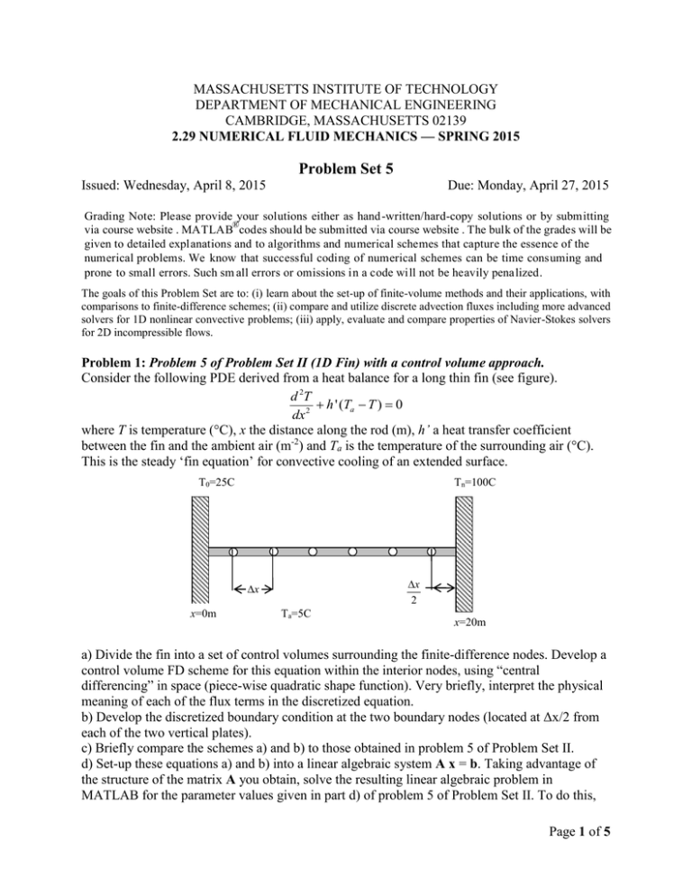
Consider the following PDE derived from a heat balance for a long thin fin (see figure).
d 2T
 h ' (Ta  T )  0
dx 2
where T is temperature (°C), x the distance along the rod (m), h’ a heat transfer coefficient
between the fin and the ambient air (m-2) and Ta is the temperature of the surrounding air (°C).
This is the steady ‘fin equation’ for convective cooling of an extended surface.
T0=25C
Tn=100C
x
x=0m
Ta=5C
x
2
x=20m
a) Divide the fin into a set of control volumes surrounding the finite-difference nodes. Develop a
control volume FD scheme for this equation within the interior nodes, using “central
differencing” in space (piece-wise quadratic shape function). Very briefly, interpret the physical
meaning of each of the flux terms in the discretized equation.
b) Develop the discretized boundary condition at the two boundary nodes (located at Δx/2 from
each of the two vertical plates).
c) Briefly compare the schemes a) and b) to those obtained in problem 5 of Problem Set II.
d) Set-up these equations a) and b) into a linear algebraic system A x = b. Taking advantage of
the structure of the matrix A you obtain, solve the resulting linear algebraic problem in
MATLAB for the parameter values given in part d) of problem 5 of Problem Set II. To do this,
Page 1 of 5
you can directly utilize the MATLAB codes that have been given to you in problem sets or
lecture, or in even MATLAB itself.
e) Optional (Bonus): only for the curious, assume that h=h’(x) varies with x and derive the
corresponding FV scheme you would obtain in c). Compare this scheme to the finite-difference
scheme you would have obtained in problem 5 of Problem Set II if h=h’(x) varied with x.
Problem 2: Burger’s equation. Burger’s equation is often referred to as the “poor man’s
Navier-Stokes equation”. It is employed to illustrate idealized nonlinear fluid processes (e.g.
steepening of waves, turbulence), and it is frequently utilized to evaluate new schemes for
handling non-linear fluxes. It is given by:
u 1 (u 2 )

0.
t 2 x
a) Using the chain-rule, evaluate the spatial derivative, and compare the re-written equation to
u
u
c
 0 . From your answer, discuss how you expect the
the Sommerfeld Wave equation
t
x
solution to behave for: i) u( x, t  0)  0 , ii) u( x, t  0)  0 .
Some fluid solutions idealized by Burger’s equation are sketched here:
b) Develop a control volume FV scheme for this equation assuming uniform discretization of the
interior nodes. Let u be a constant on each control volume. For the flux terms u2 at the edges of
control volumes, use i) Central fluxes, ii) Upwind fluxes, iii) QUICK fluxes, iv) following
fluxes:
2
f j 1/ 2
2
 u j  u j 1 
 u j  u j 1 
 u j  u j 1 
 u j 1  u j 

  max(| u j |,| u j 1 |) 

  max(| u j |,| u j 1 |) 
, f j 1/ 2  
 2 
 2 
 2 
 2 
[These latter fluxes are a “Roe solver” which is a particular Riemann solver, for details
see Leveque, 2002].
c) Implement your scheme on a periodic domain x=[0,1] with integration over the time interval
T=[0,1]. Choose an appropriate x and t so that your solution is stable. Use the following
initial conditions:
i)
ui=exp(-10*(x-0.5).^2)
ii) ui=(0.25*sin(2*pi*x')+0.5*sin(4*pi*x')+0.75)
iii) ee=0.005; %”Look-alike” Solitons
ui=( 1+0.5*(1-tanh((x'-0.3)/4/ee))-0.5*(1-tanh((x'-0.1)/4/ee)))+...
(-1+0.5*(1-tanh((x'-0.7)/4/ee))-0.5*(1-tanh((x'-0.9)/4/ee)))
Do not save every timestep, but either plot or save your solution every few timesteps. In realistic
applications, it is often not necessary to save every timestep, nor is it possible due to physical
memory constraints.
Page 2 of 5
d) Discuss your solutions (Hint: not all flux discretizations will “work”). Were your answers in
a) correct? Which flux-discretization scheme gave the best answer? How good do you think
these answers are (comment on numerical diffusion)? How do you think you could improve
these results?
Problem 3: Numerical Solution of Navier-Stokes Equations. A MATLAB code (called the 2.29
finite volume MATLAB framework) for solving the Navier-Stokes equations was provided. The
Navier-Stokes equations with Boussinesq approximation for buoyancy are as follows:
u
 u u  2u  P*  g  *kˆ  F(t , x)
[1]
t
 
  u  0 [2]
 u     2    0 [3]
t
P
'
where, P*  ,
*  ,
 '  0
0
0
The solvers used are based on several projection methods (For a review, see Guermond, J.L.,
Minev, P., and Shen, Jie. (2006). An overview of projection methods for incompressible flows.
Comput. Methods Appl. Mech. Eng., 195:6011-6045).
In this problem you are asked to run the code, compare various schemes to each other, and tie
together some of what you have learned in 2.29. To do this, you will have to use the “TestCase”
function in the 2.29 finite volume MATLAB framework.
First, you need to run “setup.m” to add the paths of the source codes. Then type “help TestCase”
from the MATLAB command window for a description. The first argument of the input to
“TestCase” selects a particular test problem, whereas the second argument specifies a set of
parameters via the structure variable “app”:
function [P,u,v,rho,NodeP,Nodeu,Nodev,Tsw,Ssw] = TestCase(problem, app)
The function returns the solution at the final time step. Therefore, if you just want to view the plots
and do not want the final solution, you can call “TestCase” without specifying output variables.
For example:
>>TestCase(2,app);
For some questions, you may have to set-up the following entries in the structure variable “app”:
% INPUTS:
%
Problem:
Test case number (see below)
%
app:
Application data structure. TestCase assigns
%
default values. Can contain entries such as:
%
app.Nx:
Number of control volumes in x direction
%
app.Ny:
Number of control volumes in y direction
%
app.T:
Final time (Optional)
%
app.dt:
Timestep size (Optional)
%
app.PlotIntrvl:
Number of timesteps till solution is plotted
%
app.nu:
Viscosity used in momentum equations (Optional)
%
app.nu = 1/Re
%
app.kappa:
Diffusivity used in Density equation (Optional)
%
app.NonInc:
If true (false by default), solves the equations
%
using the non-incremental projection method
Page 3 of 5
%
%
%
%
%
%
%
%
%
app.NonRot:
app.Advect:
If true (false by default), solves the equations
using the incremental projection method in the
non-rotational form
'TVD'
-- Use the Total Variation Diminishing
advection scheme (DEFAULT)
'QUICK' -- Quadratic Upwind Interpolation scheme
for Convective Kinetics
'UW'
-- Use the UpWind advection scheme
'CDS'
-- Use the Central Differencing Scheme
a) Advection schemes: Run “TestCase(2)” and compare to TestCase(3). Compare the UPWIND
and QUICK advection schemes. Include plots of the final tracer concentration in your report.
b) Lock-Exchange problem: A barrier initially separates two fluids, one denser than the other.
This barrier is removed at the start of the simulation. Run “TestCase(6,app)” with
app.Advect='UW', then app.Advect='QUICK’ and then app.Advect='TVD’. Compare the three
solutions obtained. As part of your answer, provide a plot for each of the three difference cases.
c) To test the convergence of this solver, a Lid driven cavity flow test case is given. Run
“Cavity_Convergence_Test.m” and compare the graph to the following figure from chapter
7.8 of Ferziger and Peric (2002), for the same problem. Calculate the rate of convergence for
the centerline velocity (using the finest resolution available).
© Springer. All rights reserved. This content is excluded from our Creative
Commons license. For more information, see http://ocw.mit.edu/fairuse.
Source: Fig. 7.12 from Ferziger, J., and M. Peric. Computational Methods for
Fluid Dynamics. Springer, 2002.
Page 4 of 5
d) Recall the suddenly expanding pipe problem from Problem Set 2 (see below). Calculate the
theoretical pressure difference for A1 = 1/3, A2=1, V1=1. Using our Navier-Stokes solver, we
will now compute this numerically. To run this test case, use TestCase(7,app), with:
Pressure ~ p1
p1, V1, A1
CV
p2, V2, A2
app.nu=0.001 and app.nu=0.005, where app.nu sets the value of viscosity. For each case:
i) Calculate the numerical pressure change from the suddenly expanding entrance, to the end
of the recirculation zone. (You may have to zoom in plots to see where the u-velocity reverses
direction).
ii) Compare with the analytical value and briefly comment. In particular, how do results
compare to Bernoulli’s estimate? Is the pressure at the walls behind eddies close to p1?
iii) How do the eddies vary with the Reynolds number? How does p2 vary with the distance x
along the pipe for the two different Reynolds numbers?
e) (Bonus: do this only if you are interested, you will get full credit without doing this part).
Building on part b), run “TestCase(6)” with default app and “TestCase(6,app)” with
“app.NonInc=1” and compare the final figure. A difference plot of the two cases may be useful.
What is the difference between the two solvers? What accounts for the difference between the
two solutions? Are the differences large? Why?
Page 5 of 5
MIT OpenCourseWare
http://ocw.mit.edu
2.29 Numerical Fluid Mechanics
Spring 2015
For information about citing these materials or our Terms of Use, visit: http://ocw.mit.edu/terms.