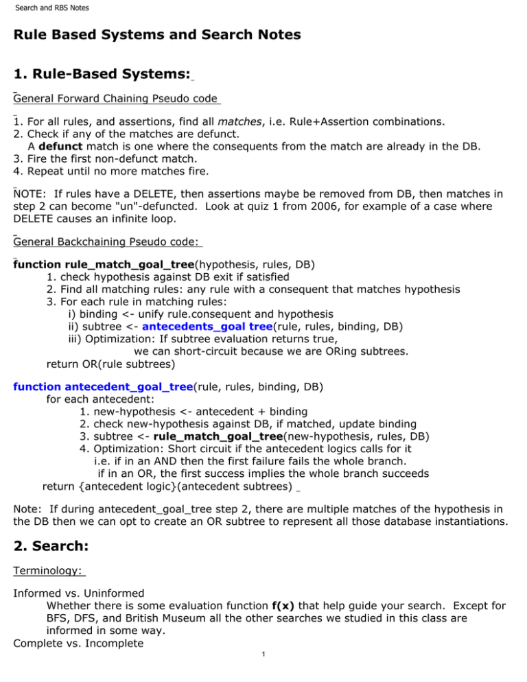
Rule Based Systems and Search Notes 1. Rule-Based Systems:
advertisement

Search and RBS Notes
Rule Based Systems and Search Notes
1. Rule-Based Systems:
General Forward Chaining Pseudo code
1. For all rules, and assertions, find all matches, i.e. Rule+Assertion combinations.
2. Check if any of the matches are defunct.
A defunct match is one where the consequents from the match are already in the DB.
3. Fire the first non-defunct match.
4. Repeat until no more matches fire.
NOTE: If rules have a DELETE, then assertions maybe be removed from DB, then matches in
step 2 can become "un"-defuncted. Look at quiz 1 from 2006, for example of a case where
DELETE causes an infinite loop.
General Backchaining Pseudo code:
function rule_match_goal_tree(hypothesis, rules, DB)
1. check hypothesis against DB exit if satisfied
2. Find all matching rules: any rule with a consequent that matches hypothesis
3. For each rule in matching rules:
i) binding <- unify rule.consequent and hypothesis
ii) subtree <- antecedents_goal tree(rule, rules, binding, DB)
iii) Optimization: If subtree evaluation returns true,
we can short-circuit because we are ORing subtrees.
return OR(rule subtrees)
function antecedent_goal_tree(rule, rules, binding, DB)
for each antecedent:
1. new-hypothesis <- antecedent + binding
2. check new-hypothesis against DB, if matched, update binding
3. subtree <- rule_match_goal_tree(new-hypothesis, rules, DB)
4. Optimization: Short circuit if the antecedent logics calls for it
i.e. if in an AND then the first failure fails the whole branch.
if in an OR, the first success implies the whole branch succeeds
return {antecedent logic}(antecedent subtrees)
Note: If during antecedent_goal_tree step 2, there are multiple matches of the hypothesis in
the DB then we can opt to create an OR subtree to represent all those database instantiations.
2. Search:
Terminology:
Informed vs. Uninformed
Whether there is some evaluation function f(x) that help guide your search. Except for
BFS, DFS, and British Museum all the other searches we studied in this class are
informed in some way.
Complete vs. Incomplete
1
Search and RBS Notes
If there exists a solution (path from s to g) the algorithm will find it.
Optimal vs. Non-optimal
The solution found is also the best one (best counted by the cost of the path).
Generic Search Algorithm:
function Search(graph, start, goal):
0. Initialize
agenda = [ [start] ]
extended_list = []
while agenda is not empty:
1. path = agenda.pop(0) # get first element from agenda & return it
2. if is-path-to-goal(path, goal)
return path
3. otherwise extend the current path if not already extended
for each connected node
make a new path (don't add paths with loops!)
4. add new paths from 3 to agenda and reorganize agenda
(algorithms differ here see table below)
fail!
The code in red only applies if you are using an extended list.
Agenda keeps track of all the paths under consideration, and the way it is maintained is
the key to the difference between most of the search algorithms.
Loops in paths: Thou shall not create or consider paths with cycles in step 3.
Extended list is the list of nodes that has undergone "extension" (step 3).
Using an extended list is an optional optimization that could be applied to all algorithms.
(some with implications, see A*) In some literature extended list is also referred to as
"closed" list, and the agenda the "open" list.
Backtracking: When we talk about DFS or DFS variants (like Hill Climbing) we talk about
with or without "backtracking". You can think of backtracking in terms of the agenda. If
we make our agenda size 1, then this is equivalent to having no backtracking. Having
agenda size > 1 means we have some partial path to go back on, and hence we can
backtrack.
Exiting the search: Non-optimal searches may actually exit when it finds or adds a path
with a goal node to the agenda (at step 3). But optimal searches must only exit when the
path is the first removed from the agenda (step 1,2).
Search Algorithm
Properties
Required Parameters
2
What is does with the
agenda in step 4.
Search and RBS Notes
Breadth-First Search
Uninformed, Nonoptimal (Exception:
Optimal only if you
are counting total
path length),
Complete
Add all new paths to
the BACK of the
agenda, like a queue
(FIFO)
Depth-First Search
Uninformed,
Non-optimal,
Incomplete
Add all new paths to
the FRONT of the
agenda, like a stack
(FILO)
Depending on
definition of f(x)
Best-First Search
If f(x) = h(x)
(estimated distance
to goal) then likely
not optimal, and
potentially
incomplete.
However, A* is a
type of best First
search that is
complete and optimal
because of its choice
of f(x) which
combines g(x) and h
(x) (see below)
n-Best-First
Non-optimal,
Incomplete
Hill Climbing
Non-optimal,
Incomplete
Like DFS with a
heuristic
3
f(x) to sort the entire
agenda by.
Keep entire agenda
sorted by f(x)
f(x) to sort the entire
agenda by. n = the
maximum size of the
agenda
Keep entire agenda
sorted by f(x) and
only keep the top n.
f(x) to sort the newly
added path by.
1. Keep only newly
added paths sorted
by f(x)
2. Add sorted new
paths to the FRONT
of agenda
Search and RBS Notes
Like BFS but expand
nodes in f(x) order.
Beam Search
Incomplete for small
k; Complete and like
BFS for k = infinity.
1. the beam width k
2. f(x) to sort the top
paths by.
Non-optimal
When k = 1, Beam
search is analogous
to Hill Climbing
without backtracking.
British Museum
Branch & Bound
Brutally exhaustive,
Uninformed,
Complete
None
Most likely
implemented using a
breadth-first
enumeration of all
paths
Optimal,
g(x) = c(s, x) = the
cost of path from s to
node x.
f(x) = g(x) + 0
Sort paths by f(x)
f(x) = g(x) + h(x,g)
h(x,g) is the estimate
of the cost from x to
g.
A* w/o extended list
(or B&B w/o
extended list +
admissible heuristic)
A* w extended list
1. Keep only k-top
paths that are of
length n. (So keep a
sorted list of paths
for every path length)
2. Keep only top-k
paths as sorted by f
(x)
Optimal if h is
admissible
Sort paths by f(x)
h(x) must be an
admissible heuristic
f(x) = g(x) + h(x)
Optimal if h is
consistent
h(x) must be a
consistent heuristic
Sort paths by f(x)
NOTE: A* with extended list and a non-consistent heuristic may be non-optimal!!
Definitions:
f(x) is the total cost of the path that your algorithm uses to rank paths.
g(x) is the cost of the path so far.
h(x) is the (under)estimate of the remaining cost to the goal g node.
f(x) = g(x) + h(x)
c(x, y) is the actual cost to go from node x to node y.
Admissible Heuristic:
●
For all nodes x in Graph, h(x) <= c(n, g)
●
i.e. the heuristic is an underestimate of the actual cost/distance to the goal.
Consistent Heuristic:
4
Search and RBS Notes
●
●
●
For edges in an undirected graph, where m is connected to n.
❍
|h(m) - h(n)| <= c(m, n)
For edges in a directed graph n is a descendent of m or m -> n
❍
h(m) - h(n) <= c(m,n)
You can verify consistency by checking each edge and see if difference between h
values on an edge <= the actual edge cost.
Consistency implies Admissibility
If you can verify consistency, then the heuristic must be admissible.
But Admissibility does not imply Consistency!!
You can make an admissible heuristic consistent by using the Pathmax algorithm:
Pathmax in a nut shell: When you are extending nodes. If you find an edge that is not
consistent, i.e. h(m) - h(n) > c(m,n); make it consistent by setting the end h(n) heuristic
value to h(m). Hence the difference becomes 0, which is always <= c(m,n) and consistent.
Short explanation on why Admissibility must be true for A* to be optimal:
Let C* is the actual cost of the optimal path from s to g.
A* search always extend paths in order of increasing f(x), where f(x) = g(x)+h(x)
You can think of A* expanding paths on a fringe. Once it has extended some path of value f(x)
we are guaranteed that it has seen all paths lower than f(x).
If h(x) is admissible, (i.e. h(x) is an underestimate of the actual path cost to node g) then we
know that any partial path leading to the optimal path solution must have f(x) <= C*.
f(x) = g(x) + h(x) <= C*
So as we expand the fringe, we are guaranteed to extend through all partial paths leading to
the optimal path C*
However If h(x) is an overestimate, then optimality may not be guaranteed;
Because there may be a partial paths that lead to the optimal path where:
f(x) = g(x) + h(x) > C*
Because of the fringe property, such a partial paths will be visited after we visit any path with
cost C*. So we will end up by either by-passing the optimal solution and/or mistaken a nonoptimal path as the solution.
Consistency ensures that f(x) is always non-decreasing. That is if
p_1, p_2, p_3...p_n are partial paths leading to the optimal path, a consistent heuristic
ensures that f(p_1) <= f(p_2) <=....<= f(p_n). This strictly non-decreasing property or
monotonicity, ensures that once a node has been extended it is the absolute best f(x) path
out of that node; it is safe to not visit that node again.
How Different Heuristics in A* affect performance
General rule: More closely h(x) approximates the actual cost to the goal the faster A* will
find the solution (or A* will do less work extending paths).
5
Search and RBS Notes
Example:
Consider the 8 square game (source AIMA):
Solve the 8 square puzzle by sliding squares horizontally or vertically until they are in
numerical order. Use A* to find the shortest number of legal moves to get from the starting
configuration (s) to the goal game configuration (g).
This is a possible start state (s)
8
5
1
4
X
2
6
7
3
This is the goal state (g)
X
1
2
3
4
5
6
7
8
Intermediate states are generated by moving a square left, right, up or down into a free blank
square.
Admissible Heuristic h1(x): Number of Misplacements - the number of squares that are not in
the correct position. For our example h1(s,g) = 8. Since all except for 6 and 7 are in the
wrong positions.
Admissible Heuristic h2(x): Manhattan distance - number of moves needed to put each
square in the right position. For our example h2(s,g) = 4 + 2 + 1 + 1 + 2 + 2 + 0 + 0 + 3 =
15
Both Heuristics are admissible because actual number of moves to get individual squares in
the correct positions will always be more (or equal).
Number of nodes extended in A* at depth 24
Using h1:
Using h2:
39.1 k
1.6 k (faster!)
Conclusion, because h2 (Manhattan distance) is a closer approximation to actual number of
moves needed, using it causes A* to do less work, and converge to the optimal solution faster.
6
MIT OpenCourseWare
http://ocw.mit.edu
6.034 Artificial Intelligence
Fall 2010
For information about citing these materials or our Terms of Use, visit: http://ocw.mit.edu/terms.


