NAME:
18.443 Exam 3 Spring 2015
Statistics for Applications
5/7/2015
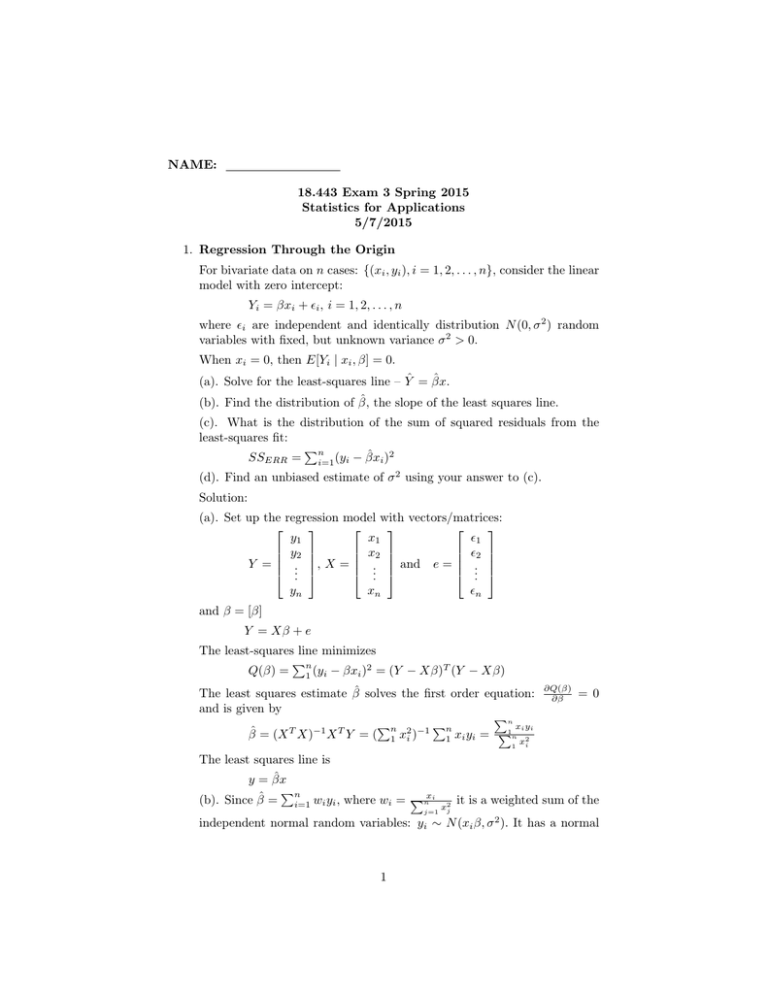
1. Regression Through the Origin
For bivariate data on n cases: {(xi , yi ), i = 1, 2, . . . , n}, consider the linear
model with zero intercept:
Yi = βxi + Ei , i = 1, 2, . . . , n
where Ei are independent and identically distribution N (0, σ 2 ) random
variables with fixed, but unknown variance σ 2 > 0.
When xi = 0, then E[Yi | xi , β] = 0.
ˆ
(a). Solve for the least-squares line – Yˆ = βx.
ˆ
the slope of the least squares line.
(b). Find the distribution of β,
(c). What is the distribution of the sum of squared residuals from the
least-squares fit:
n
i=1 (yi
SSERR =
− β̂xi )2
(d). Find an unbiased estimate of σ 2 using your answer to (c).
Solution:
(a). Set up the regression model with vectors/matrices:
⎡
⎤
⎡
⎤
⎡
⎤
y1
x1
E1
⎢ y2 ⎥
⎢ x2 ⎥
⎢ E2 ⎥
⎢
⎥
⎢
⎥
⎢
⎥
Y = ⎢ . ⎥, X = ⎢ . ⎥ and e = ⎢ . ⎥
⎣ .. ⎦
⎣ .. ⎦
⎣ .. ⎦
yn
xn
En
and β = [β]
Y = Xβ + e
The least-squares line minimizes
Q(β) =
n
1 (yi
− βxi )2 = (Y − Xβ)T (Y − Xβ)
The least squares estimate βˆ solves the first order equation:
and is given by
n
n
1
β̂ = (X T X)−1 X T Y = (
x2i )−1
n
1
xi yi =
∂Q(β)
∂β
= 0
xi yi
1
n
1
x2i
The least squares line is
ˆ
y = βx
(b). Since β̂ =
n
i=1
wi yi , where wi =
xi
n
j=1
xj2
it is a weighted sum of the
independent normal random variables: yi ∼ N (xi β, σ 2 ). It has a normal
1
distribution and all we need to do is compute the expectation and variance
of β̂:
Pn
E[β̂] = P
E[ i=1 wi yi ] P
n
n
= Pi=1 wi E[yi ] = i=1 wi × (xi β)
n
x
i
Pn 2 )xi β
=
i=1 (
x
j=1 j
2
Pn
x
= β i=1 ( Pn i x2 ) = β
j=1
V ar[β̂]
j
=
Pn
V ar[ i=1 wi yi ] P
P
n
n
2
2 2
i=1 wi V ar[yi ] =
i=1 wi σ
2
P
x
n
σ 2 × i=1 ( (Pni x2 )2 )
Pn 2 j=1 j
x
σ 2 × (Pni=1x2i)2
=
σ 2 × (Pn1
=
=
=
j=1
j
j=1
x2j )
So, β̂ ∼ N (β, σβ2 ) where σβ2 = σ 2 × (Pn1
j=1
x2j )
(c). For a normal linear regression model the distribution of the sum of
least-squares residuals has a distribution equal to σ 2 (the error variance)
times a Chi-square distribution with degrees of freedom equal to (n − p),
where p is the number of independent variables and n is the number of
cases. In this case, p = 1 so
Pn
SSERR = i=1 (yi − xi β̂)2 ∼ σ 2 χ2df =(n−1) .
(d). Since a Chi-square random variable has expectation equal to its
degrees of freedom. E[SSERR ] = σ 2 (n − 1) so
ˆ2 =
σ
SSERR
n−1
is an unbiased estiamte of σ 2 .
2. Simple Linear Regression
Consider fitting the simple linear regression model:
ŷ = β1 + β2 xi
to the following bivariate data:
i
1
2
3
4
xi
-5
-2
3
4
yi
-2
0
3
5
The following code in R fits the model:
>
>
>
>
x=c(-5,-2,3,4)
y=c(-2,0,3,5)
plot(x,y)
lmfit1<-lm(y ~ x)
2
> abline(lmfit1)
> print(summary(lmfit1))
Call:
lm(formula = y ~ x)
Residuals:
1
2
3
0.11111 -0.05556 -0.66667
4
0.61111
Coefficients:
Estimate Std. Error t value Pr(>|t|)
(Intercept) 1.50000
0.32275
4.648
0.0433 *
x
0.72222
0.08784
8.222
0.0145 *
--Signif. codes: 0 '***' 0.001 '**' 0.01 '*' 0.05 '.' 0.1 ' ' 1
0.9569
−2
−1
0
1
y
2
3
4
5
Residual standard error: 0.6455 on 2 degrees of freedom
Multiple R-squared: 0.9713,
Adjusted R-squared:
F-statistic: 67.6 on 1 and 2 DF, p-value: 0.01447
−4
−2
0
2
4
x
(a). Solve directly for the least-squares estimates of the intercept and
slope of the simple linear regression (obtain the same values as in the R
3
print summary)
Solution: The least-squares estimates are given by
β̂1
β̂2
β̂ =
⎡
1
⎢ 1
X=⎢
⎣ 1
1
= (X T X)−1 X T Y , where
⎤ ⎡
⎤
⎡
1 −5
y1
x1
⎢ 1 −2 ⎥
⎢ y2
x2 ⎥
⎥=⎢
⎥ and Y = ⎢
⎣ y3
3 ⎦
x3 ⎦ ⎣ 1
x4
1
4
y4
⎤
⎡
⎤
−2
⎥ ⎢ 0 ⎥
⎥=⎢
⎥
⎦ ⎣ 3 ⎦
5
Plugging in we get
T
−1
β̂ = (X X)
T
X Y
=
=
=
P
P4
P
−1
P yi
P1 1 P x2i
xi yi
xi
xi
−1
4 0
6
0 54
39
6/4
1.5
=
39/54
0.7222
(b). Give formulas for the least-squares estimates of β1 and β2 in terms
of the simple statistics
x = 0, and y = 1.5
sx =
Sx2 =4.2426
sy =
Sy2 =3.1091
r = Corr(x, y) =
Sxy
Sx Sy
=0.9855
Solution: We know formulas for the least-squares estimates of the slope
and intercept are given by:
Pn
√ 2
(xi −x)(yi −(y))
S
Sxy
s
1P
ˆ
√
β2 =
= S 2 = r y2 = r sxy
n
(x −x)2
1
=
β̂1
x
i
(0.9855) ×
3.1091
4.2426
Sx
= 0.7222
= y − β̂2 x
= 1.5 − (0.7222) × (0) = 1.5
(c). In the R print summary, the standard error of the slope β̂2 is given
as σ̂βˆ2 =0.0878
Using σ̂ =0.65, give a formula for this standard error, using the statistics
in (b).
Solution: We know that the variance of the slope from a simple linear
regression model (where the errors have mean zero, constant variance σ 2
and are uncorrelated) is
Pn
V ar(β̂2 ) = σ 2 / 1 (xi − x)2 = σ 2 /[(n − 1)Sx2 ]
The standard error of β̂2 is the square-root of this variance, plugging in
the estimate σ̂ for the standard deviation of the errors:
4
p
√
StErr(β̂2 ) = σ/(
ˆ
(n − 1)sx ) = 0.65/( 34.2526) = .088
(d). What is the least-squares prediction of Ŷ when X = x = 0, and what
is its standard error (estimate of its standard deviation)?
Solution: The least-squres prediction of Ŷ when X = x must be y, the
mean of the dependent variable. The simple least-squares regression line
always goes through the point of means: (x, y) = (x, y)
The standard error of this prediction is just the estimate of the standard
deviation of the sample mean y which is
q
2
σ̂y = σ̂n = √σ̂4 = 0.65/2 = 0.325
3. Suppose that grades on a midterm and final have a correlation coefficient of
0.6 and both exams have an average score of 75. and a standard deviation
of 10.
(a). If a student’s score on the midterm is 90 what would you predict her
score on the final to be?
(b). If a student’s score on the final was 75, what would you guess that
his score was on the midterm?
(c). Consider all students scoring at the 75th percentile or higher on the
midterm. What proportion of these students would you expect to be at
or above the 75th percentile of the final? (i) 75%, (ii) 50%, (iii) less than
50%, or (iv) more than 50%.
Justify your answers.
Solution:
(a). Let x be the midterm score and y be the final score. The least-squares
regression of y on x is given in terms of the standardized values:
ŷ−y
sy
= r x−x
sx
A score of 90 on the midterm is (90 − 75)/10 = 1.5 standard deviations
above the mean. The predicted score on the final will be r × 1.5 = .9
standard deviations above the mean final score, which is 75+(.9)×10 = 84.
(b). For this case we need to regress the midterm score (x) on (y). The
same argument in (a), reversing x and y leads to:
x̂−x
sx
= r y−y
sy
Since the final score was 75, which is zero-standard deviations above y,
the prediction of the midterm score is x = 75.
(c). By the regression effect we expect dependent variable scores to be
closer to their mean in standard-deviation units than the independdent
variable is to its mean, in standard-deviation units. Since the 75th per­
centile is on the midterm is above the mean, we expect these students to
have average final score which is lower than the 75th percentile (i.e., closer
to the mean). This means (iii) is the correct answer.
5
4. CAPM Model
The CAPM model was fit to model the excess returns of Exxon-Mobil (Y)
as a linear function of the excess returns of the market (X) as represented
by the S&P 500 Index.
Yi = α + βXi + Ei
where the Ei are assumed to be uncorrelated, with zero mean and constant
variance σ 2 . Using a recent 500-day analysis period the following output
was generated in R:
0.01
0.00
−0.02
−0.04
Y (Stock Excess Return)
0.02
0.03
XOM
−0.02
−0.01
0.00
0.01
0.02
X (Market Excess Return)
> print(summary(lmfit0))
Call:
lm(formula = r.daily.symbol0.0[index.window] ~ r.daily.SP500.0[index.window],
x = TRUE, y = TRUE)
Residuals:
Min
1Q
-0.038885 -0.004415
Median
0.000187
3Q
0.004445
Max
0.026748
Coefficients:
Estimate Std. Error t value Pr(>|t|)
-0.0004805 0.0003360
-1.43
0.153
(Intercept)
6
r.daily.SP500.0[index.window]
0.9190652
0.0454380
20.23
<2e-16
Residual standard error: 0.007489 on 498 degrees of freedom
Multiple R-squared: 0.451,
Adjusted R-squared: 0.4499
F-statistic: 409.1 on 1 and 498 DF, p-value: < 2.2e-16
(a). Explain the meaning of the residual standard error.
Solution: The residual standard error is an estimate of the standard devi­
ation of the error term in the regression model. It is given by
Pn
q
(yi −ŷi )2
ERR
1
σ̂ = SS
=
(n−p)
n−p
It measures the standard deviation of the difference between the actual
and fitted value of the dependent variable.
(b). What does “498 degrees of freedom” mean?
Solution: The degrees of freedom equals (n − p) where n = 500 is the
number of sample values and p = 2 is the number of regression parameters
being estimated.
(c). What is the correlation between Y (Stock Excess Return) and X
(Market Excess Return)?
√
√
Solution: The correlation is R − Squared = .451 ≈ .67
(we know it is positive because of the positive slope coefficient 0.919)
(d). Using this output, can you test whether the alpha of Exxon Mobil is
zero (consistent with asset pricing in an efficient market).
H0 : α = 0 at the significance level α = .05?
If so, conduct the test, explain any assumptions which are necessary, and
state the result of the test?
Solution: Yes, apply a t-test of H0 : intercept equals 0. R computes this
in the coefficients table and the statistic value is −1.43 with a (two-sided)
p-value of 0.153. For a nominal significance level of .05 for the test (twosided), the null hypothesis is not rejected because the p-value is higher
than the significance level. The assumptions necessary to conduct the test
are that the error terms in the regression are i.i.d. normal variables with
mean zero and constant variance σ 2 > 0. If the normal distribution doesn’t
apply, then so long as the error distribution has mean zero and constant
variance, the test is approximately approximately correct and equivalent
to using a z-test for the parameter/estimate and the CLT.)
(e). Using this output, can you test whether the β of Exxon Mobil is less
than 1, i.e., is Exxon Mobil less risky than the market:
H0 : β = 1 versus HA : β < 1.
If so, what is your test statistic; what is the approximate P -value of the
test (clearly state any assumptions you make)? Would you reject H0 in
favor of HA ?
7
Solution: Yes, we apply a one-sided t-test using the statistic:
T =
β̂−1
stErr(β̂)
=
0.919−1
0.0454
= −.081/.0454 = −1.7841
Under the null hypothesis T has a t-distribution with 498 degrees of free­
dom. This distribution is essentially the N (0, 1) distribution since the
degrees of freedom is so high. The p-value of this statistic (one-sided)
is less than 0.05 because P (Z < −1.645) = 0.05 for a Z ∼ N (0, 1) so
P (T < −1.7841) ≈ P (Z < −1.7841) which is smaller.
5. For the following batch of numbers:
5, 8, 9, 9, 11, 13, 15, 19, 19, 20, 29
(a). Make a stem-and-leaf plot of the batch.
(b). Plot the ECDF (empirical cumulative distribution function) of the
batch.
(c). Draw the Boxplot of the batch.
Solution:
> x=c(5,8,9,9,11,13,15,19,19,20,29)
> stem(x)
The decimal point is 1 digit(s) to the right of the |
0
1
1
2
2
|
|
|
|
|
5899
13
599
0
9
> plot(ecdf(x))
8
0.0
0.2
0.4
Fn(x)
0.6
0.8
1.0
ecdf(x)
5
10
15
20
x
> median(x)
[1] 13
> quantile(x,probs=.25)
25%
9
> quantile(x,probs=.75)
75%
19
> boxplot(x)
9
25
30
25
20
15
10
5
Note that the center of the box is at the median (19), the bottom is at
the 25-th percentile and top is at the 75-th percentile. The inter-quartile
range is (19-9)=10, so any value more than 1.5 × 9 = 13.5 units above or
below the box will be plotted as outliers. There are no such outliers.
6. Suppose X1 , . . . , Xn are n values sampled at random from a fixed distri­
bution:
X i = θ + Ei
where θ is a location parameter and the Ei are i.i.d. random variables with
mean zero and median zero.
(a). Give explicit definitions of 3 different estimators of the location pa­
rameter θ.
(b). For each estimator in (a), explain under what conditions it would be
expected to be better than the other two.
Solution:
(a). Consider the sample mean, the sample median, and the 10%-Trimmed
mean.
Pn
θ̂M EAN = n1 1 Xi .
θ̂M EDIAN = median(X1 , X2 , . . . , Xn )
10
θ̂T rimmedM ean = average of {Xi } after excluding the highest 10%
and the lowest 10% values.
(b). We expect the sample mean to be the best when the data are a
random sample from the same normal distribution. In this case it is the
MLE and will have lower variability than any other estimate.
We expect the same median to be the best when the data are a random
sample from the bilateral exponential distribution. In this case it is the
MLE and will hve lower variability, asymptotically than any other esti­
mate. Also, the median is robust against gross outliers in the data result­
ing from the possibility of sampling distribution including a contamination
component.
We expect the trimmed mean to be best when the chance of gross errors
in the data are such that no more than 10% of the highest and 10% of the
lowest could be such gross errors/outliers. For this estimate to be better
than the median, it must be that the information in the mean of the re­
maining values (80% untrimmed) is more than the median. This would be
the case if 80% of the data values came from a normal distribution/model.
arise from a normal distribution with
11
Percentiles of the Normal and t Distributions
N(0,1)
t (df=1)
t (df=2)
t (df=3)
t (df=4)
t (df=5)
t (df=6)
t (df=7)
t (df=8)
t (df=9)
t (df=10)
t (df=25)
t (df=50)
t (df=100)
t (df=500)
q 0.5
0.00
0.00
0.00
0.00
0.00
0.00
0.00
0.00
0.00
0.00
0.00
0.00
0.00
0.00
0.00
q 0.75
0.67
1.00
0.82
0.76
0.74
0.73
0.72
0.71
0.71
0.70
0.70
0.68
0.68
0.68
0.67
q 0.9
1.28
3.08
1.89
1.64
1.53
1.48
1.44
1.41
1.40
1.38
1.37
1.32
1.30
1.29
1.28
12
q 0.95
1.64
6.31
2.92
2.35
2.13
2.02
1.94
1.89
1.86
1.83
1.81
1.71
1.68
1.66
1.65
q 0.99
2.33
31.82
6.96
4.54
3.75
3.36
3.14
3.00
2.90
2.82
2.76
2.49
2.40
2.36
2.33
q 0.999
3.09
318.31
22.33
10.21
7.17
5.89
5.21
4.79
4.50
4.30
4.14
3.45
3.26
3.17
3.11
MIT OpenCourseWare
http://ocw.mit.edu
18.443 Statistics for Applications
Spring 2015
For information about citing these materials or our Terms of Use, visit: http://ocw.mit.edu/terms.