90
2. T IM E D O M A IN M E T H O D S
8. Trend Determination
A common debate in climate and other studies concerns the reality of trends in data. Specifically,
one is concerned that an apparent linear or more complex trend should be distinguished, as secular, from
local apparent trends which are nothing but the expected short-term behavior of a stochastic process.
The synthetic time series displayed above show extended periods where one might be fooled into inferring
a trend in climate, when it is nothing but a temporary structure occurring from pure happenstance. For
geophysical problems, the existence of rednoise time series makes the problem quite di!cult.
Suppose one has a stationary time series {t whose power density and corresponding autocovariance
U ( ) are known. From U ( ) we can make a covariance matrix as in (1.16). We suspect that superimposed
upon this time series is a linear secular trend representable as |t = d + et and we would like to determine
d> e and their uncertainty. Generalizing the discussion in Wunsch (1996, p.188), we regard {t now as a
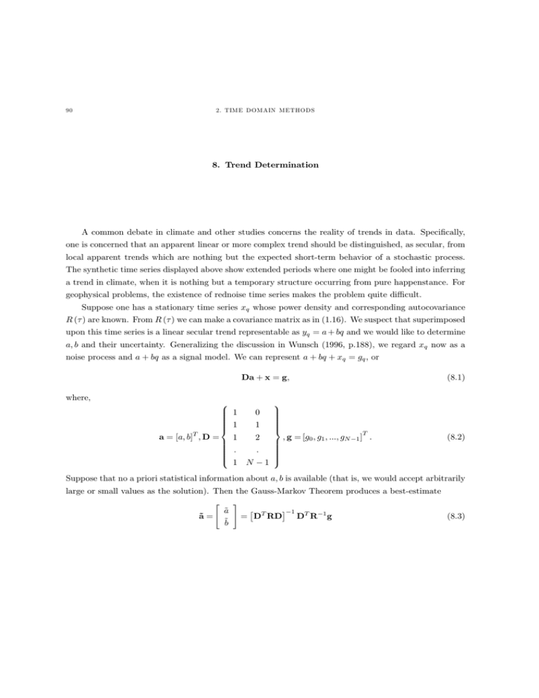
noise process and d + et as a signal model. We can represent d + et + {t = jt > or
Da + x = g>
where,
a = [d> e] > D =
W
;
A
1
A
A
A
A
A
A 1
?
0
1
1
2
A
A
A
A
=
=
A
A
A
= 1 Q 1
<
A
A
A
A
A
A
A
@
A
A
A
A
A
A
A
>
> g = [j0 > j1 > ===> jQ 1 ]W =
(8.1)
(8.2)
Suppose that no a priori statistical information about d> e is available (that is, we would accept arbitrarily
large or small values as the solution). Then the Gauss-Markov Theorem produces a best-estimate
"
#
¤1 W 1
£
˜
d
D R g
(8.3)
˜
a=
= DW RD
ẽ
91
with uncertainty
¡
¢1
=
P =? (˜
a a)2 A= DW R1 D
(8.4)
Clearly P depends directly upon the covariance R= If long-temporal correlations are present, apparent,
but spurious trends, will probably be found. But the result (8.3) will have large expected uncertainties
given by (8.4) and one would not be misled.
Exercise. Generate a time series with power density (v) = 1@(5@4 + cos (2v)). Add a known trend,
and then determine it from the above expressions.