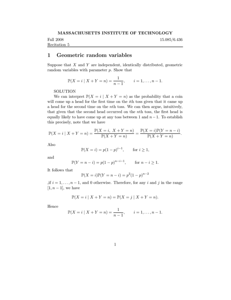
MASSACHUSETTS INSTITUTE OF TECHNOLOGY
Fall 2008
Recitation 5
1
15.085/6.436
Geometric random variables
Suppose that X and Y are independent, identically distributed, geometric
random variables with parameter p. Show that
P(X = i | X + Y = n) =
1
,
n−1
i = 1, . . . , n − 1.
SOLUTION
We can interpret P(X = i | X + Y = n) as the probability that a coin
will come up a head for the first time on the ith toss given that it came up
a head for the second time on the nth toss. We can then argue, intuitively,
that given that the second head occurred on the nth toss, the first head is
equally likely to have come up at any toss between 1 and n − 1. To establish
this precisely, note that we have
P(X = i | X + Y = n) =
P(X = i, X + Y = n)
P(X = i)P(Y = n − i)
=
.
P(X + Y = n)
P(X + Y = n)
Also
P(X = i) = p(1 − p)i−1 ,
for i � 1,
and
P(Y = n − i) = p(1 − p)n−i−1 ,
for n − i � 1.
It follows that
P(X = i)P(Y = n − i) = p2 (1 − p)n−2
,if i = 1, . . . , n − 1, and 0 otherwise. Therefore, for any i and j in the range
[1, n − 1], we have
P(X = i | X + Y = n) = P(X = j | X + Y = n).
Hence
P(X = i | X + Y = n) =
1
,
n−1
1
i = 1, . . . , n − 1.
2
Expectation of ratios
Let X1 , X2 , . . . , Xn be independent identically distributed random variables.
Show that, if m � n, then E(Sm /Sn ) = m/n, where Sm = X1 + · · · + Xm .
Solution: By linearity of expectation, we have
��n
� �
n
i=1 Xi
1=E
=
E(Xi /Sn ).
Sn
i=1
By symmetry (since the Xi are identically distributed) we must have that
E(Xi /Sn ) = E(Xj /Sn ), and thus, by the equality above, this must equal
1/n. Therefore, again appealing to the linearity of expectation, we have
�
�
m
�
Sm
E
=
E(Xi /Sn )
Sn
i=1
= mE(X1 /Sn ) = m/n.
3
Inequalities
Some inequalities that will be very useful through this course are listed
below.
Markov’s Inequality: Suppose X is a nonnegative random variable. For
a > 0, P(X > a) � E|X|/a.
Proof: Consider the random variable Y = aI X>a . Since Y � X, and both
X, Y are always positive,
E[Y ] � E[X]
But since E[Y ] = aP (X > a), we have
P (X > a) �
E[X]
a
which completes the proof.
Note that since |X| is always nonnegative, for any a > 0, and any random
variable X,
E[|X|]
P (|X| > a) �
a
Similarly, we can take apply the inequality to a 2 and X 2 to get
P (X 2 > a2 ) �
2
E[X 2 ]
a2
Since for a > 0 X 2 > a2 if and only if |X| > a,
P (|X| > a) �
E[X 2 ]
a2
for positive a.
Finally, we can take Y = (X−E[X]). Then, Markov’s inequality becomes
P ((X − E[X])2 > a2 ) �
or
�2
a2
�2
a2
The last equation is known as Chebyshev’s inequality.
Observe that we can apply Markov’s inequality to |X − E[X]| k to obtain,
P (|X − E[X]| > a) �
P (|X − E[X| > a) �
E|X − E[X]|k
,
ak
which tells us that if the k-th central moment exists (i.e. E|X −E[X]| k < →)
moment exists, we can use it to get that P (|X −E[X]| > a) decays as a −k . A
consequence is that if all the central moments exist, (i.e. E|X − E[X]| k < →
for ll k), then P (|X − E[X]| > a) decays to 0 as a � +→ faster than any
polynomial in a−1 .
4
Numerical integration through sampling
Suppose we are interested in computing
� b
g(x)dx.
a
If X is uniform over [0, 1] note that
E[g(X)] =
�
b
g(x)
a
1
dx,
b−a
so that
E[(b − a)g(X)] =
�
b
g(x)dx.
a
To compute the integral of g numerically, we can generate uniform samples
Xi over the interval a, b and compute the ratio
n
�
1
(b − a)
g(Xi ).
n
i=1
3
�b
This is an unbiased estimate of a g(x)dx.
Let us work out a simple example.�Suppose we have the function f (x) =
2
x/2. We are interested in estimating 0 f (x). Clearly, the answer is 1.
The above technique suggests using the estimator
n
X̂ =
1 �
2
Xi ,
n
i=1
where Xi are iid U (0, 2) samples. The expectation of the answer is 1/2.
Since E[Xi2 ] = 4/3, we get that the variance of this estimator is
var(X̂) = E[X̂ 2 ] − E[X̂]2 =
1 4
1
( n + n(n − 1)) − 1 =
2
n 3
3n
4
MIT OpenCourseWare
http://ocw.mit.edu
6.436J / 15.085J Fundamentals of Probability
Fall 2008
For information about citing these materials or our Terms of Use, visit: http://ocw.mit.edu/terms.