1.2.3 Pivoting Techniques in Gaussian Elimination
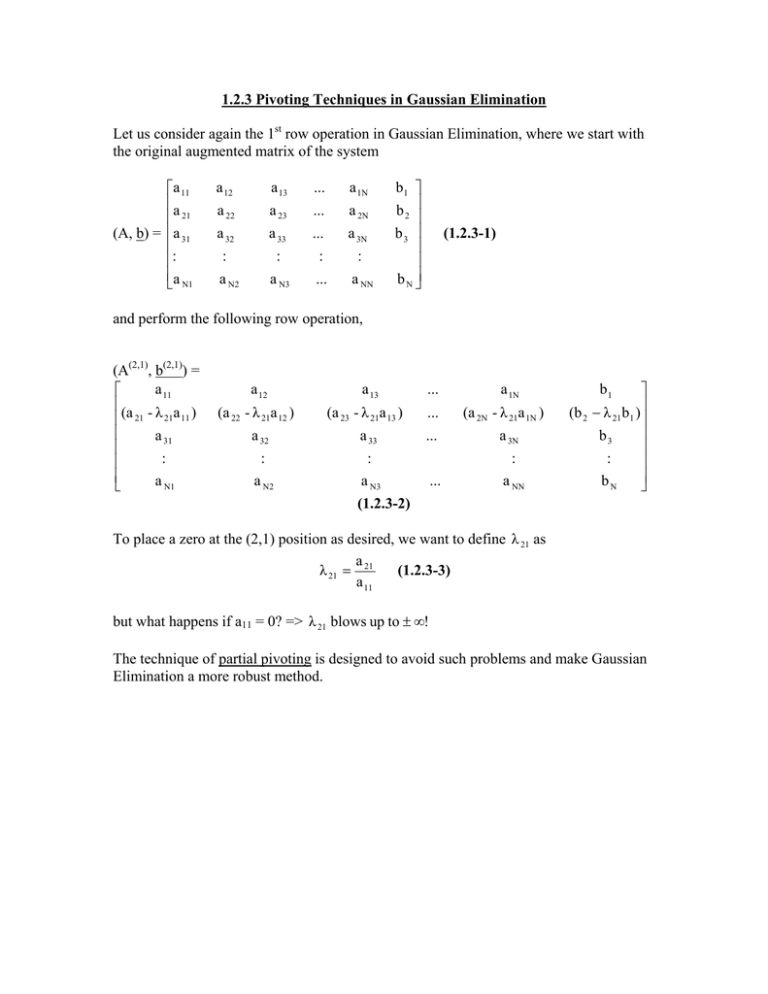
Let us consider again the 1st row operation in Gaussian Elimination, where we start with
the original augmented matrix of the system
a 11
a
 21
(A, b) = a 31

:
a N1

a 12
a 13
...
a 1N
a 22
a 23
...
a 2N
a 32
a 33
...
a 3N
:
:
:
:
a N3
...
a NN
a N2
b1 
b 2 
b3 


b N 
(1.2.3-1)
and perform the following row operation,
(A(2,1), b(2,1)) =
a 11

(a - λ a )
 21 21 11

a 31

:


a N1

a 12
a 13
...
(a 22 - λ 21a 12 )
(a 23 - λ 21a 13 )
...
a 32
a 33
...
:
:
a N2
a N3
(1.2.3-2)
a 1N
(a 2N - λ 21a 1N )
a 3N
:
...
a NN

(b 2 − λ 21 b1 )

b3

:


bN

b1
To place a zero at the (2,1) position as desired, we want to define λ 21 as
a
(1.2.3-3)
λ 21 = 21
a 11
but what happens if a11 = 0? => λ 21 blows up to ± ∞!
The technique of partial pivoting is designed to avoid such problems and make Gaussian
Elimination a more robust method.
Let us first examine the elements of the 1st column of A,
a 11 
a 
 21 
a 
A(: , 1) =  31 
: 
: 
 
a N1 
(1.2.3-4)
Let us search all the elements of this column to find the row #j that contains the value
with the largest magnitude, i.e.
a ji ≥ a k1 for all k = 1, 2, ..., N
or
a j1 = max k∈[1, N] { a k1 }
(1.2.3-5)
(1.2.3-6)
Since the order of the equations does not matter, we are perfectly free to exchange rows
# 1 and j to form the system
a j1

a 21
( A, b) = a 11

:
a
 N1
a j2
a j3
...
a jN
a 22
a 23
...
a 2N
a 12
a 13
...
a 1N
:
a N2
:
a N3
:
...
:
a NN
bj 

b2 
b1 


b N 
row # j
row # 1
(1.2.3-7)
Now, as long as any of the elements of the 1st column of A are non-zero, aj1 is non-zero
and we are safe to begin eliminating the values below the diagonal in the 1st column.
If all the elements of the 1st column are zero, we immediately see that no equation in the
system makes reference to the unknown x, and so there is no unique solution. We
therefore stop the elimination process at this point and “give up”.
The row-swapping procedure outlined in (1.2.3-1), (1.2.3-6), (1.2.3-7) is known as a
partial pivoting operation.
For every new column in a Gaussian Elimination process, we 1st perform a partial pivot
to ensure a non-zero value in the diagonal element before zeroing the values below.
The Gaussian Elimination algorithm, modified to include partial pivoting, is
For i= 1, 2, …, N-1
% iterate over columns
select row j > i such that a ji = max j≥i { a ii , a i +1,i ,..., a N,i }
if aji = 0, no unique solution exists, STOP
if j ≠ i, interchange rows i and j
For j = i+1, i+2, …, N % rows in column i below diagonal
a ji
>λ ←
a ii
For k = i, i+1, …, N % elements in row j from left
>ajk ajk - λa ik
end
>bj bj - λb i
end
right
end
Backward substitution then proceeds, in the same manner as before.
Even if rows must be swapped at each column, computational overhead of partial
pivoting is low, and gain in robustness is large!
To demonstrate how Gaussian Elimination with partial pivoting is performed, let us
consider the system of equations with the augmented matrix
1 1 1 4 
2 1 3 7

(A, b) = 
3 1 6 2 
pivot
(1.2.3-8)
First, we examine the elements in the 1st column to see that the element of largest
magnitude is found in row #3.
We therefore perform a partial pivot to interchange rows 1 and 3.
3 1 6 2 
(A, b) = 2 1 3 7 
1 1 1 4 
(1.2.3-9)
We now perform a row operation to zero the (2,1) element
λ 21 =
a 21 2
=
a 11 3
 3

2
(2,1)
(A (2,1) , b ) = 2 −  3
 3

 1
(1.2.3-10)
1
6
2
1 −  1
3
1
3 1 6 2 

1
2
= 0
1 5 
3
3

1 1 1 4 


2
3 −  6
3
1
(1.2.3-11)
We now perform another row operation to zero the (3,1) element
λ 31
(2,1)
a 31
1
= (2,1) =
3
a 11
(1.2.3-12)


2
7 −  2
3 

4

2

 3


(3,1)
(3,1)
(A , b ) =  0

1 -  1 3
  3 

3

= 0


0

1
1
3
2
3
1
6
1
3
1 
1 -  1
3 

2 

2
5
3
1
3 
3
6
-1
-1
-1
1 
1 -  6
3 


2

2

5

3

1  
4 -  2
 3  
(1.2.3-13)
We now move to the 2nd column, and note that the element of largest magnitude appears
in the 3rd row. We therefore perform a partial pivot to swap rows 2 and 3.

3

-(3,1)
(A -(3,1) , b
) = 0


0

1
2
3
1
3
6
-1
-1

2 

1
3 
3
2
5 
3
(1.2.3-14)
We now perform a row operation to zero the (3,2) element.
1
1
(1.2.3-15)
λ 32 = 3 =
2 2
3

3
1
6

2

(3,2)
(A (3,2) , b ) = 0
-1
3

1 12
1
0
-  
- 1 - (− 1)

3 23
2


2

1

3

3

2 1  1 
5 - 3 
3 2  3  

3

= 0


0

1
2
3
0
6
-1
−
1
2

2 

1
3 
3

4 

(1.2.3-16)
After the elimination method, we have an upper triangular form that is easy to solve by
backward substitution.
We write out the system of equations,
3x1 + x2 + 6x3 = 2
2
1
x2 − x3 = 3
3
3
1
− x3 = 4
2
(1.2.3-17)
First, we find
x 3 = −8
(1.2.3-18)
Then, from the 2nd equation,
1
(3 + x3 )
x2 = 32
= −7
3
(1.2.3-19)
st
And finally from the 1 equation
x1 =
(2 − 6x 3 − x2 )
= 19
3
(1.2.3-20)
The solution is therefore
19 
x =  −7
 −8
(1.2.3-21)
Note that in our partial pivoting algorithm, we swap rows to make sure that the largest
magnitude element in each column at and below the diagonal is found in the diagonal
position. We do this even if the diagonal element is non-zero.
This may seem like wasted effort, but there is a very good reason to do so. It reduces the
"round-off error" in the final answer. To see why, we must consider briefly how numbers
are stored in a computer's memory.
If we were to look at the memory in a computer, we would find data represented digitally
as a sequence of 0'a and 1's
00100101 00101011 , …..
----------- ------------byte # i
byte # i+1
To store a real number in memory, we need to represent it in such format. This is done
using floating point notation.
Let f be a real number that we want to store in memory. We do so by representing it as
some value
~
f≈f
That we write as
~
f = ±[d 1 ∗ 2 e −1 + d2 ∗ 2e −2 + ...d t ∗ 2 e −t ]
t= machine precision
(1.2.3-22)
Each
d i = 0 or 1
And so is represented by one bit in memory. e is an integer exponent in the range
L ≤e≤ U
L ≡ underflow limit
U = overflow limit
(1.2.3-23)
e is also stored as a binary number, for example if we allocate a byte (8 bits) to storing e,
then
± 0 0 0 0 0 1 1
=3
e 7 e 6 e 5 e 4 e 3 e 2 e1 e 0
(1.2.3-24)&(1.2.3-25)
The largest e is when
0
1
= e26 +=e13 ∗ 2 3 + e 4 ∗ 24 + e 5 ∗ 25 + e 6 ∗2 6
e = e 0 ∗e20 =+ e11 =
∗ 2e2 +=e...2 ∗2
For which
e max = 2 0 + 21 + 22 + 2 3 + 24 + 25 + 2 6 = ∑ k=20k = 2 7 − 1
6
(1.2.3-26)
So, say in general
k
e max ≈ 2
Where k depends on number of bits allocated to store e.
(1.2.3-27)
For the largest magnitude variable that can be stored in memory, M
M=
0
1 1 1 1 1 1 1
± d1 =1 d 2 d 3 d 4 d 5 d 6 d 7 d 8
0 1 1 1 1 1 1
± e 6 e 5 e 4 e 3 e 2 e1
[
M = + 2 e −1 + 2 e − 2 + 2 e −3 + 2 e − 4 + 2 e −5 + 2 e −6 + 2 e −7 + 2 e −8
]
(1.2.3-34)
(1.2.3-35)
where
e = +2 6 = +64
(1.2.3-36)
so
8
M = ∑ 2 e − k = 1.8375x1019
(1.2.3-37)
k =1
In general, for machine precision t and = 2k,
i
t
t
t
1 t 1
1
M = ∑ 2 U −i = 2 U ∑ 2 −i = 2 U ∑   = 2 U  ∑  
 2  i =1  2 
i =1
i =1
i =1  2 
We now use the identity for a geometric progression,
x N −1
N
i −1
∑i=1 x = x − 1 , x ≠ 1 (1.2.3-39)
i −1
(1.2.3-38)
to write
t
1
  −1
U12
M =2  
= 2U 1 − 2 − t
(1.2.3-40)
 2   1 − 1


2 
We see that, for a given t and k (i.e. how much memory we wish to allocate to storing
each number), there is a maximum and minimum magnitude to the real numbers that can
be represented.
[
]
~
m≤ f ≤M
For t = 8, for various k, U = 2k, we have the following m and M,
k
4
6
8
U=2k=-L
16
64
256
m = 2L-1
~ 7.36x10-6
~ 2.71x10-20
~ 4.32x10-78
M = 2U(1-2-t)
~ 6.53x104
~1.84x1019
~ 1.15x1077
The typical representation on a 32-bit machine is
__
+/-
__ __ __ __ __ __ __ __
8 bit exponent
__
+/-
__ __ __ __ __ __ __ __ __ __ __ __ __ __ __ __ __ __ __ __ __ __ __
23 bit mantissa
total = 32 bits for each real number
The important point to note is that when we wish to store a real number f in memory, in
general f cannot be exactly represented by a finite set of bits in floating point notation;
1
certainly this is true for , π , e . Instead, we represent it with the closest possible value
3
~
[
f = ± d1 ∗ 2 e −1 + d 2 ∗ 2 e − 2 + ...d t ∗ 2 e −t
]
(1.2.3-22, repeated)
~
so that the difference between the “true” value of f and the represented value f is called
the round-off error, rd(f)
~
rd ( f ) = f − f
(1.2.3-41)
For binary representation of a number f with m ≤ f ≤ M , from (1.2.3-22), we see that
the magnitude of the round-off error is
rd ( f ) ~ 2 e −t = 2 −t ∗ 2 e = (eps) ∗ 2 e
(1.2.3-42)
where we define the machine precision as
(eps) = 2-t, see MATLAB command “eps”
(1.2.3-43)
Let us write rd(f) = rf(eps)x2ef
(1.2.3-44)
Where
rf is some number of O(1) (i.e. is on the order of 1)
ef = exponent of f
~
We write f = m f x2 ef , where mf = mantissa of f, also O(1)
(1.2.3-45)
Then,
rd(f)
~
=
f
~
For eps << 1, rd(f) << f
rf
r
2 ef
(eps)x e f = f (eps)
mf
mf
2
(1.2.3-46)
(1.2.3-47)
So, when we initially assign a value in memory, the round-off error may be small. We
want to make sure that this initial small error, as it propagates through our algorithms,
does not “blow up” to become large.
For example, let us take the difference of two close, large numbers
f = 3.000 0001x106
g = 3.000 00009x106
(1.2.3-48)
f-g = 0.01 so f − g << f , g
~
~
If f = f + rd(f), g = g + rd(g)
(1.2.3-49)
(1.2.3-50)
~
~
f − g = f − g + [rd(f) − rd(g)]
(1.2.3-51)
so
rd(f-g) = rd(f) – rd(g)
(1.2.3-52)
Let us write
rd(f) = rf(eps)x2ef,
~
rd(g) = rg(eps)x2eg
~
e
f = m f x2 ,
g = m g x2
eg
(1.2.3-53)
(1.2.3-54)
then
~
~
rd(f − g)
~
rf (eps)2 ef − rg (eps)2
=
~
m f 2 ef − m g 2
f−g
eg
(1.2.3-55)
eg
Let us now take the case of numbers like
f = 3.000 0001x106
g = 3.000 00009x106 (1.2.3-48, repeated)
for which, in binary or decimal notation, ef = eg and mf – mg << 1
Then
~
~
rd(f − g)
~
~
=
(r
f−g
f
− rg )(eps)
mf − mg
(1.2.3-56)
as (rf-rg) = O(1) mf – mg << 1, we see that compared to
rd(f)
~
=
f
~
rf
(eps)
mf
~
rd(f − g )
~
~
f−g
>>
(1.2.3-46, repeated)
rd(f) rd(g)
, ~
~
f
g
(1.2.3-57)
Taking the difference between two large, similar numbers therefore is bad, from the view
of propagation of error, since the accumulated round-off error in the result is much larger
than it should be from a direct assignment.
We wish to design, and operate, our algorithms so that the accumulated round-off errors
do not grow larger, and ideally decay to zero. If error “blows up”, the errors become
larger in magnitude than the values that we are trying to represent, and we get instability
that crashes the program.
For example, let us say that we wish to perform the operation
a ← a − λb (1.2.3-58)
We really perform the operation on their floating point representations
~
~
~ ~
a ← a− λ b
(1.2.3-59)
~
Since rd (a ) = a − a , we subtract these equations
~ ~
rd (a ) ← rd (a ) − λb + λ b + enew
(1.2.3-60)
rd (a ) ← rd (a ) − λrd (b) + enew
(1.2.3-61)
~
If λ = λ , we can write
If λ > 1, any round-off error in b is magnified during this operation, but if λ < 1, then
error accumulated to date by b is decreased as it is “passed” to the new value of a.
In Gaussian elimination, we perform a number of operations
a jk ← a jk − λaik , λ =
a ji
aii
(1.2.3-62)
By performing partial pivoting, we ensure aii > a ji , so λ < 1 and the algorithm has
favorable error propagation characteristics.
We can further enhance this favorable property of error propagation by performing
complete, or full, pivoting.
In complete pivoting, one searches for the maximum magnitude element not only in the
current column, but in others as well. The pivoting involves not merely interchange of
rows, but also of columns. This makes the book keeping more complex as column
interchange implies an interchange of the values of the unknowns in their position in the
solution vector x. While full pivoting improves the accuracy of calculation, by more
rapidly decaying the round-off error, it is not strictly necessary for systems that are wellbalanced, i.e. all elements along any given row ai1, ai2…,aiN are all of the same order of
magnitude. We therefore do not discuss this technique further.
We now note that with the addition of partial pivoting, Gaussian elimination provides a
robust method of solving linear equations that is easily implemented by a computer. It
either returns a solution to the linear system, or, if no non-zero pivot element if found, it
recognizes that there is no unique solution and STOP’s.
We therefore have a dependable method that can be used in higher-level algorithms to
solve non-linear algebraic equations, partial differential equations, etc. First, we must
examine in closer detail the existence and uniqueness of solutions.