Remote Sensing
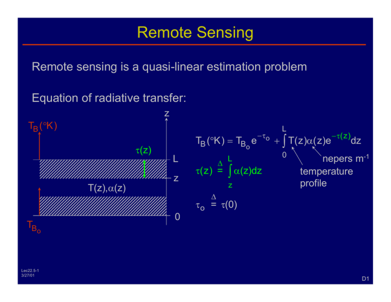
Remote sensing is a quasi-linear estimation problem
Equation of radiative transfer:
z
TB (°K )
τ(z)
T(z),α(z)
TB (°K ) = TB e
−τo
o
L
z
∆
τ(z) =
L
∫ α(z)dz
z
L
+ ∫ T(z)α(z)e
0
−τ(z)
dz
nepers m-1
temperature
profile
∆
τo = τ(0)
TB
0
o
Lec22.5-1
3/27/01
D1
Radiation from Sky-Illuminated Reflective Surfaces
TS
TB
z
1
L
2
4
0
TG
terms
3
R=1-ε
reflectivity
TB (°K ) = RTs e
−2 τo
+εTG e
sky temperature
emissivity
(specular surface)
+ Re
L
−τo
−τo
+
1 + 3
ground temperature
L
∫ T(z)α( z)e
− ∫0z α (z)dz
dz
2
0
+ ∫ T(z )α(z)e
− ∫zL α (z)dz
dz
4
0
L
Lec22.5-2
3/27/01
≅ ∫ T(z) ⎡α(z)e
⎣
0
−τ(z)
⎤ dz for τo >> 1
⎦
4
D2
Temperature Weighting Function W(z,f,T)
Terms:
1 , 2 , 3
For τo >> 1:
4
L
TB (f )
≅ To + ∫ T(z)W ( z,f,T(z)) dz
0
L
Alternatively, TB (f )
≅ To′ + ∫ ( T(z ) − To (z )) W ' ( z,f,To (z )) dz
0
Incremental weighting function:
∂TB
W ' ( z,f,To (z)) =
∂T(z ) T (z )
o
Note: we have ~linear relation:
T(z)
TB (f ) ↔
(not Fourier)
Lec22.5-3
3/27/01
D3
Atmospheric Temperature T(z) Retrievals from Space
α(ω)
(single P)
αo
∆ω ∝ pressure P
area ∝ # molecules m
2
f
ωo
Therefore α o ≠ f(P) for P-broadening trace constituents
L
TB ≅ ∫ T(z) ⎡α(z)e
⎣
z
−τ(z)
⎤ dz for τo >> 1
⎦
0
altitudes where intrinsic &
doppler broadening dominate
ω ≅ ωo
ωo ± ∆
W(z,f)
Lec22.5-4
3/27/01
pressure dominates ∆ω
ωo ± 2∆
0
α(z)
D4
Atmospheric Temperature T(z) Retrievals from Space
z
altitudes where intrinsic &
doppler broadening dominate
ω ≅ ωo
pressure dominates ∆ω
ωo ± ∆
ωo ± 2∆
L
−τ(z)
⎤ dz for τo >> 1
TB ≅ ∫ T(z ) ⎡d(z )e
⎣
⎦
α(z)
0
W(z,f)
0
z
α(ω)
∆ω
increasing P
ωo
Lec22.5-5
3/27/01
ω
f
τ≅1
scale height
W(f,z)
D5
Atmospheric Temperature T(z) Retrievals from Below
L
ωo
ωo ± ∆
W(f,z)
ωo
α(z)
0
W( f, z ) = α(z)e
− ∫0L α (z)dz
~decaying exponentials, rate is fastest for ωo
Temperature profile retrievals in semi-transparent solids or liquids where
(1/α) >> λ:
z
transparency,
If α(z) ≅ constant:
frequency dependent
L
Lec22.5-6
3/27/01
0
W(f,z)
D6
Atmospheric Composition Profiles
L
TB ≅
∫
0
α(z)
− ∫zL α(z)dz ⎤
⎡
dz
ρ(z)
• T( z)e
⎢⎣ ρ(z)
⎥⎦
W(z,f)
L
= TBo + ∫ [ρ(z) − ρo ( z)] Wρ′ ( z, f )dz
0
if viewed from space
Because α(z) and W(z,f) are strong functions of the unknown
ρ(z), this retrieval problem is quite non-linear and can be
singular (e.g. if T(z) = constant). In this case, good statistics
can be helpful. Incremental weighting functions defined relative
to a nearly normal ρ(z) can help linearize the problem.
Lec22.5-7
3/27/01
D7
Optimum Linear Estimates (Linear Regression)
Parameter vector estimate
pˆ = Dd
“determination matrix”
(d = [1,d ,..., d ])
∆
1
N
data vector
Choose D to minimize E ⎡(pˆ − p ) (pˆ − p )⎤
⎣
Derive D :
t
{
∂ E ⎡(pˆ − p )t (pˆ − p )⎤ = 0 =
⎣
⎦
∂Dij
(
t t
t
∂
⎡
=
E d D −p
∂Dij ⎣
Therefore
⎦
i
TH
row of D
⎤ = E ⎡2d D j d − 2d p ⎤
−
Dd
p
(
)
j i⎦
) ⎦ ⎣ j
DiE [dd j ] = E [pid j ]
t t
t
t
t
⎡
⎤
⎡
⎤
DE dd
= E pd ; Cd D = E ⎡dp ⎤
⎣ ⎦
⎣ ⎦
⎣
⎦
∆
Lec22.5-8
3/27/01
= Cd
F1
Optimum Linear Estimates (Linear Regression)
Therefore
DiE [dd j ] = E [pid j ]
t t
t
t
t
⎡
⎤
⎡
⎤
⎡
DE dd
= E pd ; Cd D = E dp ⎤
⎣ ⎦
⎣ ⎦
⎣
⎦
∆
= Cd
t
The linear regression solution is pˆ = Dd where D = ⎡⎣Cd ⎤⎦
Lec22.5-9
3/27/01
−1
t⎤
⎡
E dp
⎣ ⎦
F2
D is Least-Square-Error Optimum if:
1) Jointly Gaussian process (physics + instrument):
pr (r ) =
Λ
m
1
( 2π)N 2 Λ 1 2
∆
(
− 1 ⎡(r −m) Λ
⎢
e 2⎣
−1
(r −m)⎤⎥
⎦
)
t
t
= E ⎡(r − m) r − m ⎤
⎣
⎦
∆
= E ⎡⎣r ⎤⎦, where r = r1,r2,...,rN
2) Problem is linear:
data d = Mr + n + do
parameter vector
Lec22.5-10
3/27/01
noise (JGRVZM)
F3
Examples of Linear Regression
p̂
1 − D : pˆ = [D11D12 ] ⎡1 ⎤
slope = D13
p̂
regression
plane
⎢⎣d⎥⎦
D11
slope = D12
D11
0
slope = D12
d1
d
d2
note change
in slope
Equivalently:
p̂ = p + D12 ( d − d
)
(E [•] ≡ • )
Lec22.5-11
3/27/01
F4
Regression Information
1) The instrument alone (via weighting functions)
2) “Uncovered information (to which the instrument is blind,
but which is correlated with properties the instrument
does see; D retrieves this too.)
3) “Hidden information (invisible in instrument and
uncorrelated with visible information); it is lost.
Lec22.5-12
3/27/01
G1
Nature of Instrument-Provided Information
Assume linear physics: d = WT
Where
d
= data vector [1,d1,d2,...,dN ]
T
= temperature profile [T1,T2 ,...,TM ]
W = weighting function matrix
W i = ith row of W
Claim:
N
If T = ∑ ai W i and noise n = 0,
i =1
then Tˆ = Dd = T, perfect retrieval (if W not singular )
Lec22.5-13
3/27/01
G2
Proof for Continuous Variables
Claim:
N
If T = ∑ ai W i and noise n = 0,
i =1
then Tˆ = Dd = T, perfect retrieval (if W not singular )
Let:
W1(h)
∆
= b11φ1(h)
∆
W2 (h) = b21φ1(h) + b22φ2 (h)
∆
W3 (h) = b31φ1(n) + b32φ2 (h) + b33φ3 (h)
∞
⎧0
Where: ∫ φi (h) • φ j (h)dh = δij = ⎨
⎩1
0
∆
φi;bij are known a priori (from physics). Then: d j =
Lec22.5-14
3/27/01
∞
∫ T(h)W j (h)dh
0
G3
Proof for Continuous Variables
∞
∆
Then: d j =
∆
∫ T(h)Wj (h)dh
W1(h)
0
W2 (h) = b21φ1(h) + b22φ2 (h)
∆ N
If we force T(h) =
∑ k jWj (h)
= b11φ1(h)
∆
i=1
Then: d j =
N ∞
∑
t
∫ (ki Wi (h)) Wj (h)dh ⇒ d = k W W = k Q
t
t
t
i=0 0
N∞
⎛ i
⎞
⎞⎛ N
∆ N
= ∑ ∫ ki ⎜ ∑ bimφm (h) ⎟ ⎜ ∑ b jnφn (h) ⎟ ( dh) = ∑ kiQ ji
⎠
⎠ ⎝ n =1
i=1 0 ⎝ m =1
i=1
Therefore
So let
Lec22.5-15
3/27/01
d = Qk where Q is a known square matrix
−1
k̂ = Q d = k where Q is non-singular
G4
Proof for Continuous Variables
N
Claim: If T = ∑ ai W i and noise n = 0,
i =1
then Tˆ = Dd = T, perfect retrieval (if W not singular )
−1
k̂ = Q d = k where Q is non-singular
So let
Then:
∆ N
ˆ
T(h)
=
N
∑ kˆ iWi (h) = ∑ kiWi (h) = T(h) (exact)
i=1
Equivalently:
So:
i =1
( ) (
∆
−1
T = Wk = W Q d = WQ
D = WQ
Q.E.D.
−1
) d = Dd
−1 ∆
= "minimum information" solution
Which is exact if T = Wk, n = 0
Lec22.5-16
3/27/01
G5
To what is an instrument blind?
W1(h)
∆
= b11φ1(h)
∆
W2 (h) = b21φ1(h) + b22φ2 (h)
An instrument is blind to T(h) components outside the space
spanned by φ1,φ2,…,φN or, equivalently, by its W1, W2,…,Wn.
By definition, the instrument is blind to any φj ⊥ Wi, for all i.
Lec22.5-17
3/27/01
H1
Statistical Methods Can Reveal “Hidden” Components
∞
N
In general, T(h) = ∑ k i Wi (h) + ∑ aiφi (h)
=1
i
1 N
+
seen by N
instrument channels
all hidden
components
Extreme case: suppose φ1(h) always accompanied by 1 φN+1(h).
2
N
N
i =1
i =1
ˆ
= ∑ k i Wi (h) = ∑ aiφi (h)
Then our present solution: T(h)
(
)
N
Would become: T̂(h) = a1 φ1 + 1 φN+1 + ∑ aiφi
2
i= 2
shrinks with
decorrelation
Lec22.5-18
3/27/01
Thus hidden components can be
“uncovered” if correlated with visible ones.
H2
General Linear Estimate
∆
= β
i
−1⎤
∞
T̂ = Dd where Di = ⎡WQ
+ ∑ aijφ j
⎢⎣
⎥⎦i
j =N+1
minimum “uncovered”
information information
Thus retrieval can be drawn only from the space spanned by
N
⎛
⎞
φ1, φ2 ,..., φN; β1,β2 ,...,βN ⎜ dimensionality is N; Tˆ = ∑ di Di ⎟
⎝
⎠
i=1
That is, N channels contribute N orthogonal basis functions
to the minimum-information solution, plus N more basis
functions which are orthogonal but correlated with the first N.
Lec22.5-19
3/27/01
H3
General Linear Estimate
As N increases, the fraction of the hidden space which is
“uncovered” by statistics is therefore likely to increase, even
as the hidden space shrinks.
In general:
a priori variance = observed + uncovered + variance lost
due to noise and decorrelation.
Example: 8 channels of AMSU versus 4 channels of MSU
Lec22.5-20
3/27/01
AMSU and MSU are passive microwave spectrometers
in earth orbit sounding atmospheric temperature profiles
from above with ~10-km wide weighting functions
peaking at altitudes from 3 to 26 km. Note the larger
ratio of uncovered/lost power for AMSU.
H4
Example: 8-Channel AMSU vs 4-Channel MSU
MID-LATITUDES (TOTAL POWER = 1222 K2, 15 LEVELS)
OBSERVED POWER
UNCOVERED POWER
LOST POWER
MSU - 55° INCIDENCE ANGLE, LAND
MSU - 0° ANGLE, NADIR
AMSU - NADIR
AMSU - NADIR
3 km WEIGTHING FUNCTION
TROPICS (TOTAL POWER = 184
MSU – NADIR, LAND
10
6 12 22 26
16
(WINDOW)
K2)
UNCOVERED
LOST
AMSU - NADIR
0
Lec22.5-21
3/27/01
10
20
30
40
50
60
PERCENT POWER
70
80
90
100
H5