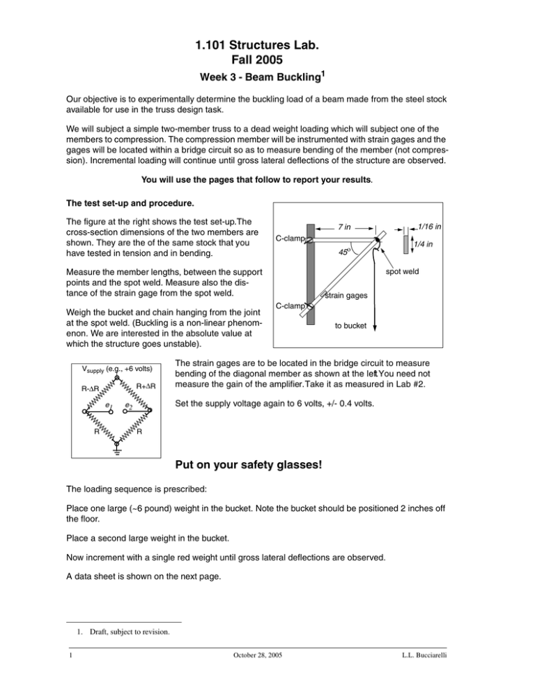
1.101 Structures Lab.
Fall 2005
Week 3 - Beam Buckling1
Our objective is to experimentally determine the buckling load of a beam made from the steel stock
available for use in the truss design task.
We will subject a simple two-member truss to a dead weight loading which will subject one of the
members to compression. The compression member will be instrumented with strain gages and the
gages will be located within a bridge circuit so as to measure bending of the member (not compres­
sion). Incremental loading will continue until gross lateral deflections of the structure are observed.
You will use the pages that follow to report your results.
The test set-up and procedure.
The figure at the right shows the test set-up.The
cross-section dimensions of the two members are
shown. They are the of the same stock that you
have tested in tension and in bending.
Vsupply (e.g., +6 volts)
R+∆R
R-∆R
e1
R
1/4 in
45o
spot weld
Measure the member lengths, between the support
points and the spot weld. Measure also the dis­
tance of the strain gage from the spot weld.
Weigh the bucket and chain hanging from the joint
at the spot weld. (Buckling is a non-linear phenom­
enon. We are interested in the absolute value at
which the structure goes unstable).
1/16 in
7 in
C-clamp
strain gages
C-clamp
to bucket
The strain gages are to be located in the bridge circuit to measure
bending of the diagonal member as shown at the left.You need not
measure the gain of the amplifier.Take it as measured in Lab #2.
Set the supply voltage again to 6 volts, +/- 0.4 volts.
e2
R
Put on your safety glasses!
The loading sequence is prescribed: Place one large (~6 pound) weight in the bucket. Note the bucket should be positioned 2 inches off the floor.
Place a second large weight in the bucket.
Now increment with a single red weight until gross lateral deflections are observed. A data sheet is shown on the next page.
1. Draft, subject to revision.
1
October 28, 2005
L.L. Bucciarelli
TEST 1. Buckling Test Data
Load
op-amp output
type
+/­
Total Load
Strain
(in bending).
lbs.
Bending
Moment
in-lb.
+/­
+/­
+/­
+/­
Column 2
Column 3
Column 4
Column 5
Bucket&Chain
.. plus 1 Big Wt.
.. plus 1 Big Wt.
.. plus 1 Red Wt.
.. plus 1 Red Wt.
“
“
“
Column 1
Columns 1 and 2 are measured data. Column 1 is the load, by load type (Big weight, Red weight);
Column 2 is the op-amp output.
Column 3 is the total accumulated load at any stage, including the weight of the bucket and chain.
Column 4, the strain, is obtained from the sequence of relationships that relate the strain to the frac­
tional change in resistance to the output of the bridge to the output of the op-amp as in last week’s
bending test.
Column 5 is the bending moment at the location of the strain gages. From Appendix A, we have
σ
My ⋅ z
--- = -------ε xx = -----xx
-----E
EI
2
hence
2EI ⋅ ε xx
M y = ------------------­h
October 28, 2005
L.L. Bucciarelli
Bending Moment My
in-lb.
Plot the bending moment versus the applied load.
Total Load (Bucket+chain+weights - lbs.)
Discuss:
3
October 28, 2005
L.L. Bucciarelli
Appendix A
Engineering Beam Theory
For a beam loaded symmetrically with respect to
mid-span as shown, the applied loads engender a
“bending moment” distribution, My(x) and a “shear
force” distribution, Qz(x), over the length of the
beam. The convention for positive force and
moment, in accord with 1.050, is shown in the fig­
ure. Not shown are the two vertical reactions at the
points of simply-support. Each is equal in magni­
tude to F.
L
z,
F
a
c
F
c
a
x
Qz
F
Note that the shear force and bending moment dis­
tributions satisfy the equilibrium requirements:
-F
dQ z
= 0
dx
z
dM y
– Qz = 0
dx
Qz
My
My
x
In writing the first of these, which guarantees force
equilibrium in the vertical direction, we have
neglected the (uniformly distributed) weight of the
beam itself.
My=- a*F
Note that over the mid-section of the beam, the
shear force is zero and the bending moment constant. We say this section is in “pure bending”. The
bending moment within the mid-section -c< x <+c, is the product of the distance a and the force F
(as shown in class).
Engineering beam theory shows that the most
significant stress is the normal stress compo­
nent on an “x face”; σxx in the example at the
right. It is related to the bending moment by
σ xx
∫z
2
z
Qz
My
x
M ⋅z
= ------y------­I
F
In this equation, z is the distance from the
“neutral axis” which, for a doubly symmetric
beam, is at the center of the cross-section and
I is the “moment of inertia” of the cross section
I =
σxx
L
z,
F
a
a
x
dA
A
z
For a rectangular cross-section of width b and height h, this is I = bh3/12
h
b
The shear force engenders a shear stress, σzx which distributes over the face, directed in the verti­
cal direction (not shown) but this is of a smaller order of magnitude. We will also neglect its effect on
the displacement of the beam.
4
October 28, 2005
L.L. Bucciarelli
The extensional strain component, εxx, under the same set of assumptions, is simply proportional to
the normal stress component,
σxx..
σ xx M y ⋅ z
- = ------------­ε xx = ------E
EI
For our beam, with its doubly symmetric cross-section, the (compressive) strain at the top of the
beam is equal in magnitude to the (tensile) strain at the bottom of the beam. This justifies our place­
ment of the strain gages in the Wheatstone bridge.
From the geometry of deformation, the exten­
sional strain is given by
F
ε xx = – z ⁄ R
L
z,
a
w(x)
F
a
x
where R is the radius of curvature of the axis. (1/
R) is the curvature. The negative sign is neces­
sary since we take the curvature, 1/R, to be posi­
tive when the beam bends concave upwards.
From the last two relationships we see that the
bending moment is related to the radius of curva­
ture at any point along the span by
1
– M y = M b = ( EI ) ⋅  --­
R
R
Mb.
Mb= - My
(Please excuse the introduction of Mb).
The curvature, for small deflections, is related
to the vertical displacement of the axis of the
beam by, (1/R) = d2w/dx2.
Finally, an integration of the differential equation obtained from the moment curvature relation gives,
taking account of the boundary conditions that the displacement at the supports must vanish, for
the mid-span deflection
w
midspan
2
2
Fa
= –  ------------ ⋅ (3 L – 4 a )
 24 EI
NOTE: F is one half of the load added to the chain below the table surface.
5
October 28, 2005
L.L. Bucciarelli
Appendix B. - The bridge circuit.
The “Wheatstone bridge” produces an output voltage proportional to the change in resistance of the
active strain gages. This voltage signal, in turn, is input into an operational amplifier, which boosts
the (dc) signal by a factor, the Gain factor. We analyze the bridge circuit anew since the placement
of the gages in the bridge circuit differs from last week.
The two strain gages fixed to the specimen subject to loading are
positioned as shown. The figure indicates that the active gage
located top left is the gage fastened to the top surface of the
beam. It is subject to compression, hence its resistance
decreases. The active gage located top right in the figure is fas­
tened to the bottom surface of the beam and experiences tension.
Note: It does not matter if you switch the location of the two
active gages in the bridge circuit. This will just change the
polarity of the voltage difference between e1 and e2.
As before, we use two “in-active” gages for temperature compen­
sation. We apply the circuit laws to determine the output voltage
e1 - e2 as a function of ∆R/R.
Vsupply (e.g., +6 volts)
R-∆R
R+∆R
i
e1
e2
i
R
R
Consider the current flow through the two resistors on the left side
of the bridge. From the usual circuit laws, we have.
V supply – e 1 = i ⋅ ( R – ∆R)
V supply
e 1 = ---------------------------­
(2 – ∆ R ⁄ R)
which yields
e1 – 0 = i ⋅ ( R ) The same kind of analysis gives, for the current flow through the two resistors on the right:
V supply
e 2 = ---------------------------­
(2 + ∆ R ⁄ R)
The output of the bridge, the voltage difference e1 - e2
.e 1
is then
(2 + ∆ R ⁄ R ) – (2 – ∆ R ⁄ R)
2 ⋅ (∆ R ⁄ R)
– e 2 = V supply ⋅ ---------------------------------------------------------------- = ------------------------------------V supply
2
(2 + ∆ R ⁄ R ) ⋅ (2 – ∆R ⁄ R)
[4 – (∆ R ⁄ R) ]
But the ratio (∆R/R)2 is going to be much less than 1.0, so we neglect this ratio with respect to 4.0 in
the denominator and obtain the same relationship as in our tension test:
V supply
e 1 – e 2 = ----------------(
∆ R ⁄ R)
2
The change in resistance is proportional to the strain, that is
∆ R ⁄
R = Fgage ε
where the gage factor is 2.07 So knowing the output voltage (difference) e1 -
e2 we can use these last two equations to determine the strain, ε. The voltage (difference) e1 - e2 is
obtained from the output of the op-amp, reduced by the Gain factor, i.e., e1 - e2 = (Op-amp output)/
(Op-amp Gain)
6
October 28, 2005
L.L. Bucciarelli
Appendix C. - Notes on the use of a spreadsheet.
You are encouraged to make use of a spreadsheet in processing your data and presentation of your
results. However, if you choose to do so, you must make sure you remain in control of your presen­
tation and make clear all steps in your data reduction and analysis. Be careful to:
• Include only the number of significant figures you can justify;
• Label all columns;
• Make explicit on the spreadsheet itself, or in text that accompanies the spreadsheet, the relationships that relate one column to another.
• On a graph generated by the spreadsheet, label all axes, showing units as well as
values at points along the axes that will enable a reader to easily read the plot;
• Draw a line (or curve if the behavior is non linear) through the points plotted. Show
your estimate of uncertainty in the location of points. • Do not rely upon color to differentiate among different plots on the same graph. (Unless you want to go to the expense of printing out the graph in color);
• In most cases, the spreadsheet reduction and analysis of data belongs in an appen­
dix. The graph of results, on the other hand, usually goes in the results section of the main body of a report1. 1. In the structure labs 1 and 2, you are not required to write a full report but only “fill in the
blanks” of the handout. If you use a spreadsheet you may insert the spreadsheet at the appropri­
ate place in the handout.Your design task will be documented differently- to be explained in
class.
7
October 28, 2005
L.L. Bucciarelli