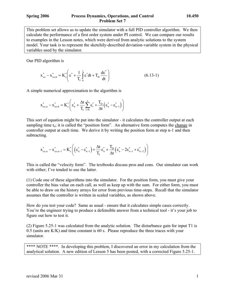
Spring 2006
Process Dynamics, Operations, and Control
Problem Set 7
10.450
This problem set allows us to update the simulator with a full PID controller algorithm. We then
calculate the performance of a first order system under PI control. We can compare our results
to examples in the Lesson notes, which were derived from analytic solutions to the system
model. Your task is to represent the sketchily-described deviation-variable system in the physical
variables used by the simulator.
Our PID algorithm is
x −x
*
co
*
co , b
⎛ * 1 t *
dε * ⎞
⎟
⎜
= K ⎜ ε + ∫ ε dt + TD
⎟
T
dt
I 0
⎠
⎝
*
c
(6.13-1)
A simple numerical approximation to the algorithm is
⎛
⎞
T
Δt n
x *co,n − x *co,b = K*c ⎜ ε*n + ∑ ε*i + D ε*n − ε*n −1 ⎟
TI i =0
Δt
⎝
⎠
(
)
This sort of equation might be put into the simulator - it calculates the controller output at each
sampling time tn; it is called the “position form”. An alternative form computes the change in
controller output at each time. We derive it by writing the position form at step n-1 and then
subtracting.
⎛
⎞
T
Δt
x *co,n − x *co,n −1 = K*c ⎜ ε*n − ε*n −1 + ε*n + D ε*n − 2ε*n −1 + ε*n −2 ⎟
TI
Δt
⎝
⎠
(
)
(
)
This is called the “velocity form”. The textbooks discuss pros and cons. Our simulator can work
with either; I’ve tended to use the latter.
(1) Code one of these algorithms into the simulator. For the position form, you must give your
controller the bias value on each call, as well as keep up with the sum. For either form, you must
be able to draw on the history arrays for error from previous time-steps. Recall that the simulator
assumes that the controller is written in scaled variables, as shown above.
How do you test your code? Same as usual - ensure that it calculates simple cases correctly.
You’re the engineer trying to produce a defensible answer from a technical tool - it’s your job to
figure out how to test it.
(2) Figure 5.25-1 was calculated from the analytic solution. The disturbance gain for input T1 is
0.5 (units are K/K) and time constant is 60 s. Please reproduce the three traces with your
simulator.
**** NOTE ****. In developing this problem, I discovered an error in my calculation from the
analytical solution. A new edition of Lesson 5 has been posted, with a corrected Figure 5.25-1.
revised 2006 Mar 31
1