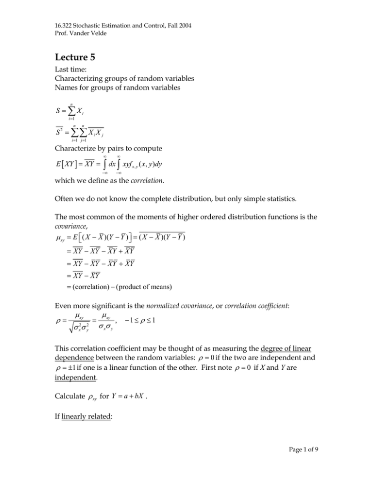
16.322 Stochastic Estimation and Control, Fall 2004
Prof. Vander Velde
Lecture 5
Last time: Characterizing groups of random variables Names for groups of random variables n
S = ∑ Xi
i=1
n
n
S 2 = ∑∑ X i
X j
i=1 j=1
Characterize by pairs to compute
E [ XY ] = XY =
∞
∞
−∞
−∞
∫ dx ∫ xyf
x, y
( x, y )dy
which we define as the correlation.
Often we do not know the complete distribution, but only simple statistics.
The most common of the moments of higher ordered distribution functions is the
covariance,
µ xy = E ⎡(
⎣ X − X )(Y − Y )⎤⎦ = ( X − X )(Y − Y )
= XY − XY − XY + XY
= XY − XY − XY + XY
= XY − XY
= (correlation) − (product of means)
Even more significant is the normalized covariance, or correlation coefficient:
ρ =
µ xy
σ σ
2
x
2
y
=
µ xy
,
σ xσ y
−1 ≤ ρ ≤ 1
This correlation coefficient may be thought of as measuring the degree of linear
dependence between the random variables: ρ = 0 if the two are independent and
ρ = ±1 if one is a linear function of the other. First note ρ = 0 if X and Y are
independent.
Calculate ρ xy for Y = a + bX .
If linearly related:
Page 1 of 9
16.322 Stochastic Estimation and Control, Fall 2004
Prof. Vander Velde
Y = a + bX
XY = a X + b X 2
Y 2 = a 2 + 2abX + b2 X 2
aX + b X 2 − X (a + bX )
ρ=
σ x2 (a 2 + 2abX + b2 X 2 − a 2 − 2abX − b2 X 2 )
=
(
b X2 − X2
(
)
σ x2b2 X 2 − X 2
)
=
bσ x2
= ±1 = sgn(b)
bσ x2
Degree of Linear Dependence
At every observation, or trial or the experiment, we observe a pair x,y. We ask:
how well can we approximate Y as a linear function of X?
Yapprox .
= a + bX
Choose a and b to minimize the mean squared error, ε 2
, in the approximation.
ε = Yapprox.
− Y = a + bX − Y
ε 2 = a 2 + b2 X 2 + Y 2
+ 2abX − 2bXY − 2aY
= a 2 + b 2 X 2 + Y 2 + 2abX − 2b XY − 2aY
Page 2 of 9
16.322 Stochastic Estimation and Control, Fall 2004
Prof. Vander Velde
∂ε 2
= 2a + 2bX − 2Y = 0
∂a
∂ε 2
= 2b X 2 + 2aX − 2 XY = 0
∂b
∂ε 2
∂ε 2
−X
= (2b X 2 − 2 XY ) − (2bX 2 − 2 XY ) = 0
∂b
∂a
σ y
XY − XY µ xy
=
=
ρ
b= 2
2
σ x
X − X 2 σx
µ xy
σ y
=
−
ρ
X
Y
X
σ x2
σx
µ
µ
Yapprox . = Y − xy2 X + xy2 X
σx
σ x
µ
= Y + xy
(X − X )
σ x2
σ
=Y + ρ y (X − X )
σx
σ
ε = Yapprox. − Y = Y + ρ y ( X − X ) − Y
σx
ε =0
a =Y −
ε 2 = a ( a + 2bX − 2Y ) + b2 X 2 + Y 2 − 2b XY
µ
µ
µ
µ
µ
= (Y − xy2 X )(Y − xy2 X + 2 xy2 X − 2Y ) + xy2 X 2 + Y 2 − 2 xy2 XY
σx
σx
σx
σx
σx
µ
µ
µ
µ
µ
= −Y 2 + xy2 XY + xy2 XY − xy2 X 2 + xy2 X 2 + Y 2 − 2 xy2 XY
σx
σx
σx
σx
σx
= σ y2 − 2
= σ y2 −
µ xy
µ xy 2 2
µ
σ
+
σ x2 xy σ x4 x
⎛
µ xy 2
µ xy 2 ⎞
2
σ
1
=
−
y ⎜
⎜ σ x2σ y2 ⎟⎟
σ x2
⎝
⎠
= σ y2
(1 − ρ 2 )
Page 3 of 9
16.322 Stochastic Estimation and Control, Fall 2004
Prof. Vander Velde
If X and Y were actually linearly
related, the points would appear on
one straight line, ρ would be ±1 , and
the mean squared error in the
approximation would be zero.
If X and Y were independent, the
points would scatter all over the x,y
plane, µ xy would be zero, so
Yapprox . = Y , and ε 2 = σ y2 .
Note that dependence other than linear is not necessarily measured by ρ .
Example: Y = X 2 and X = X 3 = 0 .
µ xy = XY = XY = X 3 − X X 2 = 0
→ ρ = 0, but X , Y are dependent!
Also, high correlation does not imply cause and effect.
Example: Dying in the hospital.
A survey reports that two events, “entering the hospital” and “dying within 1
week” have a high correlation. This relationship, however, is not causal.
There exists a third, unreported event, “disease,” which causes each of the
other events.
Page 4 of 9
16.322 Stochastic Estimation and Control, Fall 2004
Prof. Vander Velde
Vector-Matrix Notation
Define the vectors X and x and the mean E [ X ] .
E[X ] =
∞
∞
∫ dx ... ∫ dx xf
1
−∞
n
n
( x)
−∞
⎡ x1
⎤
= ∫ dx1... ∫ dxn ⎢ M ⎥ f n ( x)
⎢ ⎥
−∞
−∞
⎢⎣ xn ⎥⎦ = X
∞
∞
⎡ X1 ⎤
⎢ ⎥
=⎢ M ⎥
⎢⎣ X n ⎥⎦
Correlation Matrix
E ⎡⎣ XX T ⎤⎦ = XX T = M
M ij = X i X j
So the correlation matrix arrays all the correlations among the Xi with the mean
squared values on the diagonal. Note that: • The correlation matrix is symmetric.
• If Xi and Xj are independent, the correlation is the product of the means
(from the product rule for the pdf).
Xi X j = Xi X j
Covariance Matrix
T
T
T
T
T
E ⎡(
⎣ X − X )( X − X ) ⎤⎦ = E ⎣⎡ XX ⎤⎦ − E [ X ] X − XE ⎣⎡ X ⎦⎤ + XX
= E ⎡⎣ XX T ⎤⎦ − XX T − XX T + XX T
= XX T − XX T ≡ C
T
Cij = ⎡(
⎣ X − X )( X − X ) ⎤⎦ij
= Xi X j − Xi X j
This is by definition the covariance between Xi and Xj. So the covariance matrix
arrays all the covariances among the Xi with the variances along the diagonal.
Page 5 of 9
16.322 Stochastic Estimation and Control, Fall 2004
Prof. Vander Velde
If Xi and Xj are independent, their covariance is zero.
If the covariance between two variables is zero, they are said to be uncorrelated.
This does not, in general, imply that they are independent.
Conditional Distribution
Sometimes the notion of a conditional distribution is important. If we wish to
confine our attention to the subject of cases in which an event E occurs, we
would define the conditional probability distribution function:
FE ( x ) = F ( x | E ) = P( X ≤ x | E )
=
P ( X ≤ x, E )
P( E )
and the conditional probability density function:
dF ( x )
f E ( x) = f ( x | E ) = E
dx
Application of Bayes’ Rule
Bayes’ theorem can be written for the distribution of a random variable
conditioned on the occurrence of an event E or the observation of a certain value
of another random variable.
Conditioned on an event E:
P( Ak ) P( E | Ak )
Original form: P( Ak | E ) =
∑ P( Ai ) P( E | Ai )
i
Let the events Ai → the events x < X ≤ x + dx
Note that for different values x as dx → 0 these events are mutually exclusive
and collectively exhaustive.
lim f ( x | E )dx =
dx→0
f ( x )dxP( E | x )
∞
∫
f (u ) P( E | u )du
−∞
f (x | E) =
f ( x ) P( E | x )
∞
∫
f (u ) P( E | u )du
−∞
Page 6 of 9
16.322 Stochastic Estimation and Control, Fall 2004
Prof. Vander Velde
Example: Measuring the position of a spacecraft far away
Measurement: y = x + n , where n is noise. E implies y lies in a quantized
interval. It is simple to use this interval to estimate y, but not correct.
E ⇒ y1
< y ≤ y2
y1
< x + n ≤ y2
y1 − x < n ≤ y2
− x
We update the unconditional distribution for x to the conditional distribution
for x. This is the right way.
Page 7 of 9 16.322 Stochastic Estimation and Control, Fall 2004
Prof. Vander Velde
Conditioned on a value of Y:
will be the value taken by y (like a
Let the event E be the event y < Y ≤ y + dy . E
measurement variable).
lim f ( x | y ) =
dy→0
f ( x ) f ( y | x)dy
∞
∫
f (u ) f ( y | u)dydu
−∞
Note: y is not the variable of integration.
f ( x) f ( y | x)
f ( x | y) = ∞
∫ f (u) f ( y | u)du
−∞
This provides a basis for the estimation of a parameter X based on prior
information, f(x), and measurements y which are related to X.
Example: y = x + n n = y − x parameterizing x
f ( y | x) = f n ( y − x )
We assume n is independent of x.
f ( y | x ) is the noise distribution shifted by x.
Conditional Expectation
The conditional expectation of a random variable or function of a random
variable is the expectation calculated with the conditional distribution.
E [ g ( x ) | A] =
∞
∫ g ( x ) f ( x | A)dx
−∞
A useful relation involving conditional expectations is
E [ g ( x )] = ∑ P( Ai ) E [ g ( X ) | Ai
]
i
if the Ai are mutually exclusive and exhaustive. Or, if we let the events Ai be the
events y < Y ≤ y + dy ,
Page 8 of 9
16.322 Stochastic Estimation and Control, Fall 2004
Prof. Vander Velde
E [ g ( x )] =
∞
∫ E [ g ( x ) | y ] f ( y )dy
−∞
The conditional expectation of a random variable, E [ x | y ] , is often taken as the
estimate of the random variable after incorporating the effect of a measured
event or related random variable.
f ( x | E1 ,..., En ) : State of knowledge about x given observations E1,…,En
f ( x | y1 ,..., yn ) : State of knowledge about x given measurements y1,…,yn
Probability Distribution of Functions of Random Variables
The probability distribution and density for functions of random variables can be
calculated from the distributions of the variables themselves.
In general, if Z = g ( X , Y ) and we want f z ( z ) , we can use
Fz ( z ) = P( Z ≤ z)
= P [ g ( X ,Y ) ≤ z ]
= ∫ dx ∫ dy f x , y ( x, y )
to get the distribution function for all values of z.
dF ( z )
f z ( z) = z
dz
In particular cases, there may be easier ways to do this, but this is the general
procedure.
Page 9 of 9